To reduce the output voltage and current ripple of the BUCK converter and minimize the power inductor, using an interleaved parallel BUCK is a good choice. This article briefly discusses the method of driving interleaved BUCKs and closed-loop control based on a digital signal processor (DSP) to provide some insights.
The basic topology is as follows:
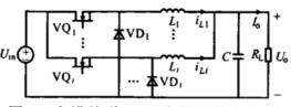
This is an interleaved BUCK using diodes for continuous current.
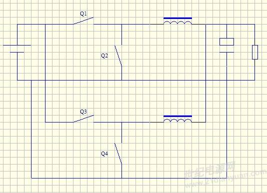
Interleaved synchronous BUCK
The following are actual waveforms:
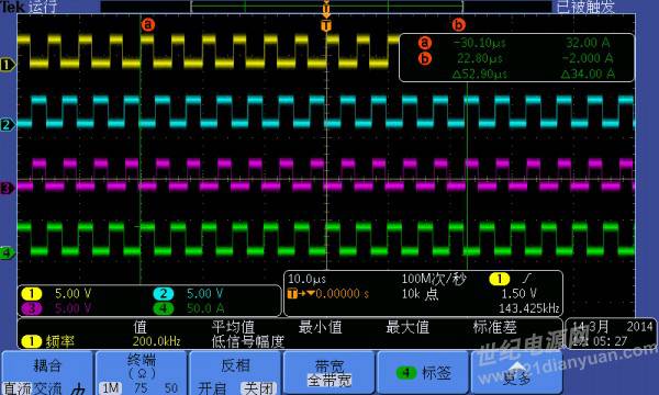
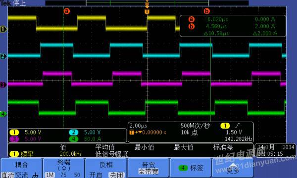
The DSP drives the interleaved configuration, where Q1 and Q2 are complementary; Q1 is the switch for BUCK1, and Q2 is the synchronous rectifier for BUCK1. Similarly, Q3 and Q4 are complementary, with Q3 being the switch for BUCK2 and Q4 being the synchronous rectifier for BUCK2.
The dead time when Q1 and Q2, as well as Q3 and Q4, are complementary is necessary. If MOSFETs are used as switching devices, a dead time of 600 ns is sufficient. For my setup with a switching frequency of 200 kHz, the dead time cannot be set too large; otherwise, the adjustable range of the duty cycle will be limited.
Additionally, note that the driving of Q2 and Q1 is 180 degrees out of phase theoretically, but in practice, there is some dead time.
This means that the maximum duty cycle cannot reach an absolute 50%, implying that the maximum duty cycle needs to be less than 50%.
The following is the waveform of the maximum duty cycle:
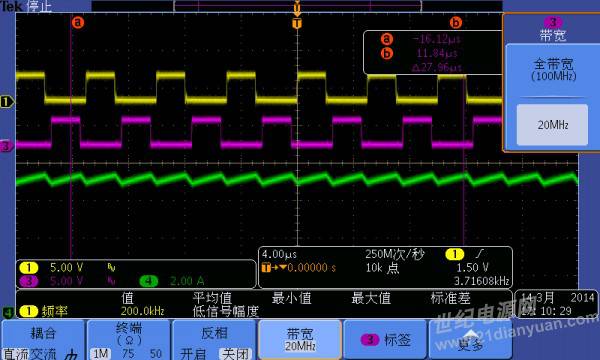
In a two-phase interleaved BUCK, the maximum duty cycle is defined as 50%. Q1 and Q3 are 180 degrees out of phase, and the maximum duty cycle is theoretically less than 50%. At this point, the variation in the output current waveform is minimized. The current waveform I tested was without the output filter capacitor, as this makes it easier to observe the changes in the current waveform.
The following waveform shows the current waveform with a small filter capacitor added, as seen in the green waveform:
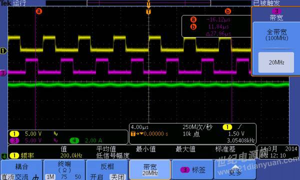
From the above figure, it can be seen that the output current frequency is twice the switching frequency, which is 400 kHz. Therefore, the power inductor can be made very small; in this example, the inductance for the two-phase interleaved setup is 5 µH.
Preston
It is suggested that the author consider a few questions:
1. Does the duty cycle of the two-phase interleaved buck theoretically need to be less than 50%? Is there a causal relationship between the current sharing and duty cycle of the two-phase buck?
2. For a fixed input voltage, is the output ripple current of a single-phase buck circuit (which equals the inductor ripple current at this time) monotonically related to the duty cycle? If it is a two-phase interleaved buck, is this relationship still monotonic?
I cannot agree with several points made by the author.
後會絠萋
I will upload a few images later tonight showing the driving waveforms and output current waveforms for two BUCKs with duty cycles of 48% and 55%, and then we can analyze them.
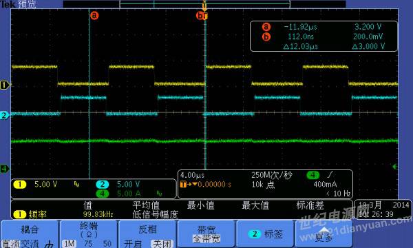
First, here are two images for everyone to look at, and then we can analyze the driving waveforms and output current waveforms when the duty cycles of the two BUCKs are close to 50% (less than 50%):
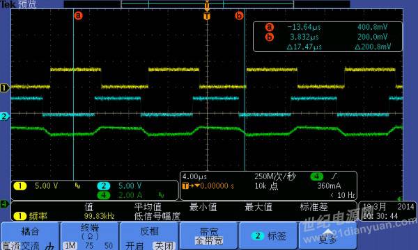
2. The driving waveforms and output current waveforms when the duty cycles of the two BUCKs exceed 50%:
Preston
The second image clearly shows that the duty cycles of the two drives are different; the yellow one is wider than the blue one. Moreover, the phase difference is not 180 degrees. When both drives are greater than 50%, there is no moment when both are low.
後會絠萋
That’s right, the yellow is slightly wider than the blue. I believe this setting with duty cycles slightly greater than 50% for the two BUCKs is to facilitate observing the changes in output current.
The first image shows a duty cycle less than 50% or close to 50%, and the current ripple is quite small, right?
While the second image shows the current waveform with a duty cycle greater than 50%, which exhibits anomalies, indicating that the two power inductors are conflicting in their energy storage and release timing.
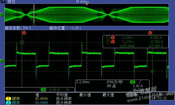
The following image shows the current commutation situation:
As can be seen, the current switching spikes still exist. The PID has been tuned for a long time, but this spike cannot be eliminated; it is caused by overshoot in the loop.
The current PID parameters are Kp=18, Ki=3, Kd=20.
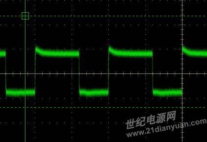
After adding feedforward:
Understanding the PID Control Algorithm
Using longitudinal control of a vehicle as an example to explain some understandings of PID.
First, why use PID?
Due to external factors, the actual speed of the vehicle is sometimes unstable, which is one reason.
To make the vehicle reach the target speed in the shortest time possible is the second reason.
The speed control system must be closed-loop to meet the stability requirements of the entire system, as speed is one of the system parameters; this is the third reason.
The speed adjustment of the vehicle is definitely not linear; there are so many external factors that no one can prove it is linear. If it were linear, we could just use P control.
For example, at PWM=60%, the speed is 2 m/s, and if you want it to be 3 m/s, you would increase the PWM to 90%. Because 90/60=3/2, this would be perfect.
Perfection is impossible.
So, if it is not linear, how do we control the PWM to achieve the desired speed? It needs to be fast, accurate, and decisive (i.e., fast, accurate, and decisive). The adjustment process of this system’s speed must be done through some algorithm, and generally, PID is the algorithm used for this purpose. You might think that if the encoder measures the current speed as 2.0 m/s and you want to reach 2.3 m/s, you could just increase the PWM a bit, right? Yes, but how much should you increase the PWM? It must be done through an algorithm because the relationship between PWM and speed is unknown for the entire system. You have to try incrementally, adding 1%; if that’s not enough, add another 1%; if that’s still not enough, you might add 2% the third time.
Through the three PID parameters, we derive an expression: △PWM=a *△V1+b *△V2+c *△V3, where a, b, c are the numbers obtained from the long PID formula after expansion and simplification, and △V1, △V2, △V3 are the speed differences after the first, second, and third adjustments, respectively. In short, PID aims to establish how to adjust the PWM and speed relationship to reach the target speed as quickly as possible.
What are the inputs and outputs?
The inputs are the previous speed, the speed before that, and the speed before that.
The output is how much your PWM should increase or decrease.
PID Control Algorithm and Its Function
The PID controller is a type of linear controller that linearly combines the proportional, integral, and derivative of the deviation between the setpoint and the actual output value to form the control quantity.
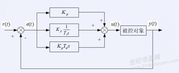
Digital PID controllers are quite mature and are sufficient for general power closed-loop control, with three parameters (Kp, Ki, Kd).
I have done practical debugging; I initially wanted to model it, but I couldn’t figure that out, so I just did it manually. I created a factory debugging interface on the upper computer for real-time debugging and observed the results with an oscilloscope, which is very convenient and intuitive.
My summarized experience with PID debugging:
First, set the current to 20% of the rated value.
1. Set I and D to zero, gradually increase P from the minimum until oscillation occurs, then lower it slightly. When it stops oscillating, remember this P value.
2. Then gradually increase I from a small value until oscillation occurs, then lower it slightly. Remember this I value. Set the current to 40% of the rated value and repeat the above steps, then 60%, 80%, and 100% of the current debugging. Often, it requires multiple iterations to find the optimal state, so patience is needed.
For more exciting content, click to read the full article! Participate in forum interactions for great rewards!

Click below“Read the original text”to see more↓↓↓