Support Vector Machine (SVM) is a supervised learning algorithm based on statistical learning theory. Its core objective is to find an optimal hyperplane in the feature space to maximize the separation between different classes of samples. This optimality is reflected in maximizing the margin, which is the distance from the support vectors (the closest sample points to the hyperplane) to the hyperplane. SVM excels at handling high-dimensional data and can effectively solve nonlinear classification problems. Even if the data is not linearly separable in the original space, SVM can map it to a high-dimensional feature space using kernel functions, thus achieving linear separability.
Before starting the tutorial, we need to install Python and Anaconda.
Anaconda is a popular Python distribution that integrates Python itself along with a large number of libraries for data science and machine learning. Installing Anaconda can save you the hassle of manually installing these libraries later.
Step 1: Download the Anaconda installer
(https://www.anaconda.com/download)
Visit the download page: Open the Anaconda official website’s download page. Choose the installer: Select the appropriate installer based on your operating system (Windows, macOS, or Linux). For Windows users, it is recommended to download the Windows 64-bit Installer (Python 3.x version).
Step 2: Install Anaconda
Run the installer: Double-click the downloaded installation file.
To confirm whether Anaconda and Python are installed successfully, please perform the following operations:
-
Open the Command Prompt (press
<span>Win + R</span>on Windows, type<span>cmd</span>and hit enter) or Terminal (macOS/Linux). -
Type the following command in the command line and hit enter:
conda --version
python --version
If the installation is successful, the version numbers of conda and Python will be displayed.
Now let’s begin the formal machine learning process!
1. Import and Split Data
# Import modules
from sklearn.datasets import load_iris
from sklearn.model_selection import train_test_split
from sklearn.preprocessing import StandardScaler  # Standardization
from sklearn.preprocessing import MinMaxScaler  # Normalization
import numpy as np
import pandas as pd

# Read Excel file
df = pd.read_excel('score_data.xlsx')

# Split data: columns 1-9 as features, column 10 as target variable
data_X = df.iloc[:, 0:9]  # First 9 columns as features
data_y = df.iloc[:, 9]    # 10th column as target variable

# Split into training and testing sets
dataX_train, X_test, y_train, y_test = train_test_split(
    data_X,
    data_y,
    test_size=0.2,
    random_state=42)

# Output training set size
print(f"Training set size: {len(X_train)}")

# Standardization
ss = StandardScaler()
X_train_standardized = ss.fit_transform(X_train)  # Standardize training set
X_test_standardized = ss.transform(X_test)        # Standardize testing set

# Normalization
mm = MinMaxScaler()
X_train_normalized = mm.fit_transform(X_train)    # Normalize training set
X_test_normalized = mm.transform(X_test)          # Normalize testing set
2. If the data is imbalanced, such as special patient data with fewer samples compared to the normal population, use the SMOTE method.
## Handling imbalanced data with SMOTE
# Find the best class
# First, import necessary modules
from sklearn.model_selection import GridSearchCV
from imblearn.pipeline import Pipeline  # Import Pipeline from imblearn
from imblearn.over_sampling import SMOTE
from sklearn.svm import SVC

# Assume you already have data X_train, y_train
# Initialize SMOTE and classifier
smote = SMOTE(random_state=42)
classifier = SVC(random_state=42)

# Use imblearn's Pipeline
pipeline = Pipeline(steps=[
    ('smote', smote),
    ('classifier', classifier)])

# Define parameter grid
param_grid = {
    'smote__k_neighbors': [3, 5, 7],
    'classifier__C': [0.1, 1, 10]}

# Create GridSearchCV object
grid_search = GridSearchCV(pipeline, param_grid, cv=5, scoring='f1_macro')  # It is recommended to use an appropriate scoring metric
grid_search.fit(X_train, y_train)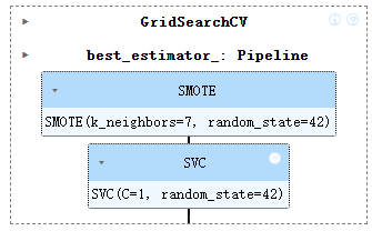
The parameter I obtained here is 7, so I will use this parameter for sample balancing.
## Handling imbalanced data with SMOTE
# Example code: Set k value
from imblearn.over_sampling import SMOTE

# Initialize SMOTE object
smote = SMOTE(k_neighbors=7, random_state=42)
# Apply SMOTE algorithm
X_train_smote, y_train_smote = smote.fit_resample(X_train, y_train)
# Check results
print('Shape of training set after balancing:', X_train_smote.shape)
print('Shape of training labels after balancing:', y_train_smote.shape)
3. Find the best parameters, hyperparameter tuning
## Hyperparameter tuning during training to find the best parameters
from sklearn.model_selection import GridSearchCV
from sklearn import svm
from sklearn.metrics import classification_report, confusion_matrix

# Define parameter grid
param_grid = {
    'C': [0.1, 1, 10, 100, 1000],
    'gamma': [1, 0.1, 0.01, 0.001, 0.0001],
    'kernel': ['rbf', 'linear', 'poly', 'sigmoid']}

# Create SVM model
svc = svm.SVC()

# Create grid search object
grid = GridSearchCV(
    estimator=svc,
    param_grid=param_grid,
    refit=True,
    verbose=3,
    cv=5,  # Number of cross-validation folds
    n_jobs=-1  # Use all available CPU cores)

# Perform grid search on training data
grid.fit(X_train_smote, y_train_smote)

# Output best parameters
print("Best parameters:", grid.best_params_)
print("Best cross-validation score:", grid.best_score_)

# Use best model for prediction
best_predictions = grid.predict(X_test)
print("Best model predictions:", best_predictions)
4. Model Prediction
## Model fitting and prediction
from sklearn import svm

# Create SVM model
clf = svm.SVC(kernel='rbf', C=1.0, gamma='scale')

# Train model
clf.fit(X_train_smote, y_train_smote)

# Predict
predictions = clf.predict(X_test)
print("Predictions:", predictions)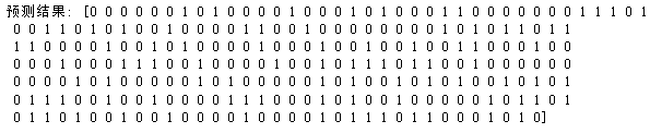
5. Model Prediction Evaluation
## Model evaluation
from sklearn.metrics import f1_score
print("F-score: {0:.2f}".format(f1_score(predictions,y_test,average='micro')))
from sklearn.metrics import classification_report, f1_score

# Generate confusion matrix
cm = confusion_matrix(y_test, predictions)
# Generate detailed evaluation report, including Precision, Recall, F1 for each class
print(classification_report(y_test, predictions))
cm
## Model evaluation
from sklearn.metrics import f1_score
print("F-score: {0:.2f}".format(f1_score(predictions,y_test,average='micro')))
from sklearn.metrics import classification_report, f1_score

# Generate confusion matrix
cm = confusion_matrix(y_test, predictions)
# Generate detailed evaluation report, including Precision, Recall, F1 for each class
print(classification_report(y_test, predictions))
cm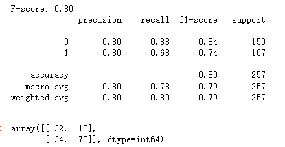
-
Precision concerns the accuracy of the predictions. The less garbage mixed in with the caught fish, the higher the precision.
-
Recall concerns the coverage of the actual situation. The fewer fish that slip through the net, the higher the recall.
-
F1-Score is a comprehensive metric that is especially useful when data is imbalanced (for example, when there are very few good samples and many bad ones). It requires both to be relatively high; any one being too low will lower the F1 score.
-
Support tells you how many samples there are in each category, which is used to measure the reliability of the metrics. If a category has only 10 samples, the calculated metrics may not be as stable as those for a category with 1000 samples.
6. Plotting the ROC Curve
## ROC Curve
from sklearn.metrics import roc_curve, auc
import numpy as np
from sklearn.svm import SVC  # Import SVC class from sklearn.svm

# Create SVC classifier instance and set probability=True
svm_classifier = SVC(probability=True, random_state=42)  # Other parameters like kernel, C, etc. can be set as needed

# Train model
svm_classifier.fit(X_train, y_train)

# Calculate prediction probabilities
y_scores = svm_classifier.predict_proba(X_test)[:, 1]

# Calculate two coordinates for the ROC curve
fpr, tpr, thresholds = roc_curve(y_test, y_scores)

# Calculate AUC value
roc_auc = auc(fpr, tpr)

# Plot ROC curve
import matplotlib.pyplot as plt
plt.figure()
lw = 2
plt.plot(fpr, tpr, color='darkorange', lw=lw, label='ROC curve (area = %0.2f)' % roc_auc)
plt.plot([0, 1], [0, 1], color='navy', lw=lw, linestyle='--')
plt.xlim([0.0, 1.0])
plt.ylim([0.0, 1.05])
plt.xlabel('False Positive Rate')
plt.ylabel('True Positive Rate')
plt.title('Receiver Operating Characteristic')
plt.legend(loc="lower right")
plt.show()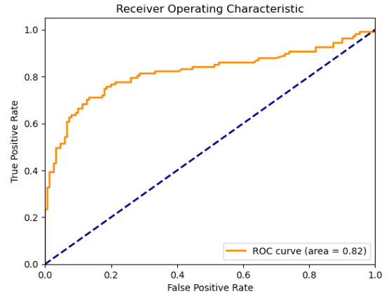
If you want sample data for this case for practical use, feel free to follow and message me~
Previous selected content: Welcome to search for more exciting content from the public account column
1. Research Methods:
Beginner’s Video Tutorial: A Step-by-Step Guide to Cross-Lagged Network Analysis (Part 1, Network Analysis)
Beginner’s Video Tutorial: A Step-by-Step Guide to Cross-Lagged Network Analysis (Part 2, Cross-Lagged Network Analysis)
Advanced Network Analysis – Complete Code for Cross-Lagged Network Analysis (CLPN): Longitudinal Network Construction
Advanced Network Analysis – Complete Code for Cross-Lagged Network Analysis (CLPN): Longitudinal Network Construction and Node Metric Analysis
Beginner’s Tutorial || Conducting Meta-Analysis Using R Code (Diagnostic Accuracy, DTA)
Beginner’s Tutorial: Conducting Latent Profile Analysis Based on R Code
Beginner’s Tutorial || Completing Confirmatory Factor Analysis and Structural Equation Modeling Based on R Code
Beginner’s Tutorial: Complete Network Analysis Based on R Code
Beginner’s Tutorial: Completing Cross-Lagged Panel Models Based on R Code
Beginner’s Tutorial || Conducting Permutation Tests Using R Language
Beginner’s Tutorial: TF-IDF Word Frequency Analysis and Topic Modeling Based on Python
Beginner’s Tutorial: Representational Similarity Analysis (RSA) of Questionnaire Data Based on R Code – Part 1
Beginner’s Tutorial: Representational Similarity Analysis (RSA) of Questionnaire Data Based on R Code – Part 2
How Beginners Can Master Artificial Intelligence (Part 5): How to Use Large Models for Automation (AI-Agent), Freeing Human Hands
How Beginners Can Master Artificial Intelligence (Part 6): How to Use Large Models for Deep Learning Tasks (Text-to-Speech, Voice Cloning, Image Recognition, etc.)
2. Study Abroad Application Section
Did not get the CSC public study abroad opportunity? There are other ways to study abroad.
How to Write the CSC External Supervisor Invitation Letter
How to Write the CSC Language Proof
How to Write the CSC Chinese Research Plan (Research Topic’s Situation in Domestic and International Studies)
3. Literature Interpretation Section
Computers in Human Behavior: Characteristics of Smartphone Use Problems Based on Intensive Longitudinal Tracking and Their Associations with Mental Health
Journal of Affective Disorders: Sleep Links College Students’ Depression and Internet Addiction – A New Perspective Based on Network Analysis
Nature Human Behaviour: Perceptual Differences and Value Preferences of Human Empathy in the Age of Artificial Intelligence
Tourism Management: The Impact Mechanism of AIGC and UGC on Tourism Decision-Making from the Perspective of Digital Confusion
Literature Interpretation: An Integrative Framework of Geography and Psychology: A Three-Dimensional Model of Interdisciplinary Interaction
Literature Interpretation: Stability of Adolescent Depression Symptom Networks – A New Perspective on Network Temperature
Literature Interpretation: How Mental Health Status Shapes Adolescents’ Social Media Behavior? – Results from a Large Sample Study