Finite State Machine (FSM), also known as a finite state machine, is a mathematical model used to represent a finite number of states and the transitions and actions between these states. It is one of the core concepts in digital logic design, particularly suitable for describing systems with clear sequential processes or those that need to respond to external events.
In FPGA design, the state machine is the soul of the control logic, responsible for coordinating the operational sequence of various modules in the datapath, acting like the command center of the control system, telling each state what to do at what time.
Three Key Elements of State Machines: States, Transition Conditions, Outputs
State machines are mainly divided into Moore and Mealy types:
a)Moore State Machine
Outputs are determined solely by the current state, independent of input signals.
Characteristics:
Outputs are stable after a state transition until the next state change.
Logic is generally simpler, and outputs do not exhibit glitches (Glitch), as outputs pass through only one layer of state registers.
Response may be “slow” by one clock cycle, as input changes require a state change first, and outputs will update in the next clock cycle.
Model: Output= F(Current State)
b)Mealy State Machine
Outputs are determined by both the current state and input signals.
Characteristics:
Responds faster to input changes, allowing outputs to change within the same clock cycle as the state transition.
Logic is more complex, and outputs may glitch due to asynchronous changes in input signals, requiring careful handling.
Outputs depend not only on the state but also on the input, making verification and debugging sometimes more complex.
Model: Output= F(Current State + Input)
How to Choose?
Use Mealy when strict timing requirements demand fast input response and effective handling of potential glitch risks.
Use Moore when seeking stable outputs and simple, reliable designs.
Often, a hybrid approach is used, where most outputs are Moore type, while a few critical outputs are Mealy
4. State Machine Encoding Methods
This is the process of mapping state names to binary values, which directly affects performance after layout and routing.
Binary Encoding:
Uses standard binary counting (e.g., 00, 01, 10, 11).
Advantages: Uses the fewest flip-flops, saving register resources.
Disadvantages: State transitions may involve multiple bits changing simultaneously (e.g., from 01->10, both bits change), leading to significant glitches and dynamic power consumption, with the lowest reliability.
Gray Code:
Only one bit changes between adjacent states (e.g., 00->01->11->10).
Advantages: Eliminates glitches and metastability risks during state transitions, with low power consumption. Very suitable for synchronizing state signals across clock domains (CDC).
Disadvantages: Requires more logic to decode states, which may complicate the logic.
One-Hot Encoding:
Each state is represented by one bit. For N states, N registers are used. At any time, only one register is ‘1’ (hot), while the others are ‘0’ (cold). For example, 4 states: 0001 (idle), 0010 (start), 0100 (run), 1000 (stop).
Advantages: Preferred in FPGA design. State decoding logic is very simple (just check which bit is 1), making it fast. FPGAs have a large number of flip-flops, while combinational logic resources are relatively scarce; this encoding trades flip-flops for better performance and simpler logic.
Disadvantages: Occupies the most flip-flop resources. For designs with a very high number of states (e.g., more than 32), it may no longer be the optimal choice.
Note: In FPGA, one-hot encoding is preferred, unless the number of states is extremely large (>32), as it usually performs better in terms of performance and area.
Below is an example of a three-stage state machine implementation for a vending machine from Nowcoder, with the problem link as follows:
https://www.nowcoder.com/exam/oj?page=1&tab=Verilog%E7%AF%87&topicId=302
First, draw the state transition diagram:
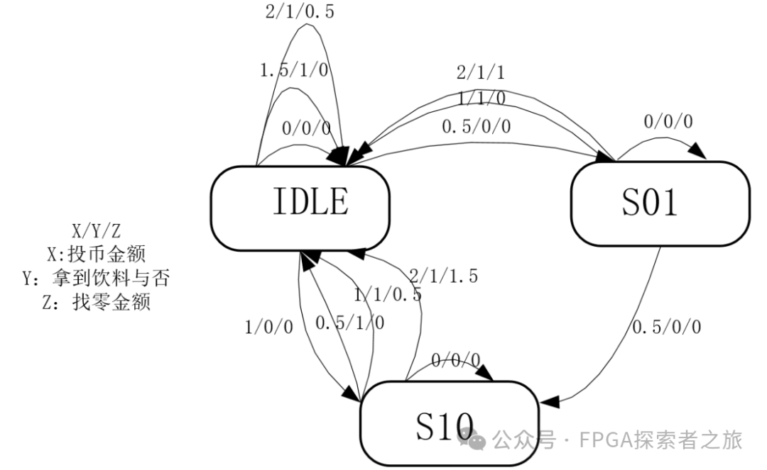
Figure 1. State Transition Diagram
Start code design (three-stage)
module state_buy(
input clk,
input rst_n,
input d1,// Coin input 0.5
input d2,// Coin input 1
input d3,// Coin input 1.5
output reg out1, //1 indicates drink dispensed, 0 indicates not dispensed
output reg [1:0] out2 //3’b00 no change, 3’b01 change 0.5, 3’b10 change 1, 3’b11 change 1.5
);
parameter IDLE=3’b001,
S01=3’b010,// Current 0.5 yuan
S10=3’b100;// Current 1 yuan
reg [2:0] cs, ns;
// Three-stage state machine first part: sequential logic describing state transitions
always@(posedge clk)
if(!rst_n)
cs <= IDLE;
else
cs <= ns;
// Three-stage state machine second part: combinational logic describing state transition conditions
always@(*)
if(!rst_n)
ns = IDLE;
else begin
case({d1,d2,d3})
3’b100:begin
if(cs==IDLE)
ns = S01;
else if(cs==S01)
ns = S10;
else
ns =IDLE;
end
3’b010:begin
if(cs==IDLE)
ns = S10;
else
ns =IDLE;
end
3’b001:ns =IDLE;
default:ns =IDLE;
endcase
end
// Three-stage state machine third part: sequential logic describing outputs
always@(posedge clk)begin
if(!rst_n)begin
out1 <= 1’b0;
out2 <= 2’d0;
end
else begin
case(cs)
IDLE:begin
if({d1,d2,d3}==3’b001)
begin
out1 <= 1’b1;
out2 <= 2’d1;
end
else begin
out1 <= 1’b0;
out2 <= 2’d0;
end
end
S01:begin
case({d1,d2,d3})
3’b100:begin
out1 <= 1’b0;
out2 <= 2’d0;
end
3’b010:begin
out1 <= 1’b1;
out2 <= 2’d0;
end
3’b001:begin
out1 <= 1’b1;
out2 <= 2’d2;
end
default:begin
out1 <= 1’b0;
out2 <= 2’d0;
end
endcase
end
S10:begin
case({d1,d2,d3})
3’b100:begin
out1 <= 1’b1;
out2 <= 2’d0;
end
3’b010:begin
out1 <= 1’b1;
out2 <= 2’d1;
end
3’b001:begin
out1 <= 1’b1;
out2 <= 2’d3;
end
default:begin
out1 <= 1’b0;
out2 <= 2’d0;
end
endcase
end
default:begin
out1 <= 1’b0;
out2 <= 2’d0;
end
endcase
end
end
endmodule
Simulation waveform as follows:
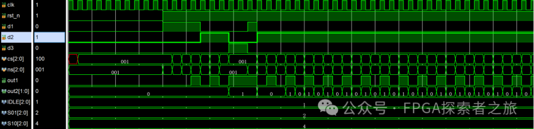
Figure 2. Simulation Waveform