Advanced Python Aggregate Modeling! Solving Overlaps, Errors, and Integrating Finite Element Analysis (Includes Optimization Code)

In the previous article, we taught you how to run a basic aggregate model using Python. We received many messages asking: “What to do if particles overlap?” “How to use the exported data?” “How to fix topology errors?”

Today, we present an advanced version focusing on three core pain points:Particle overlap, common errors, and integration with engineering software, all of which are pitfalls I have encountered along with practical solutions, including key optimization code that you can use right away!

1. Core Pain Point 1: How to Resolve Particle Overlap? Dynamic Optimization

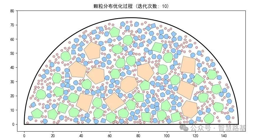
In the simplified code from the previous article, particles were placed randomly, which easily leads to overlaps (for example, two particles squeezed together), resulting in completely inaccurate subsequent mechanical analysis.

My solution is **”Dynamic Optimization”** — allowing particles to push each other away like “charged balls”. The key code and principles are as follows:

Each particle is treated as a “charged ball”; overlapping particles will generate repulsive forces, with the force increasing as the overlap area increases until they are separated.

Key code (repulsive force calculation + position update):

def optimize_overlap(self, particles, repulsion_strength=0.05, damping=0.8, max_iter=600):    """Dynamic optimization: solve particle overlap"""    for _ in range(max_iter):        total_displacement = 0  # Total displacement to determine stability        # 1. Calculate repulsive force for each particle        for i, p1 in enumerate(particles):            force = np.array([0.0, 0.0])  # Initialize force            for j, p2 in enumerate(particles):                if i == j:                    continue  # Skip self                # Quick check: if distance is too far, no need to calculate overlap                dist = np.linalg.norm(p1.position - p2.position)                min_dist = (p1.base_size + p2.base_size)/2 * 1.05  # Safe distance                if dist > min_dist:                    continue                # Detailed calculation of overlap area (using shapely library)                from shapely.geometry import Polygon as ShapelyPoly                poly1 = ShapelyPoly(p1.transformed_vertices)                poly2 = ShapelyPoly(p2.transformed_vertices)                if poly1.intersects(poly2):                    overlap_area = poly1.intersection(poly2).area                    # Magnitude of repulsive force: overlap area × strength coefficient                    force_mag = repulsion_strength * overlap_area * 10                    # Direction of repulsive force: from p2 to p1 (pushing away)                    dir_vec = p1.position - p2.position                    if np.linalg.norm(dir_vec) < 1e-6:                        dir_vec = np.random.normal(0, 1, 2)  # Avoid division by zero                    dir_vec = dir_vec / np.linalg.norm(dir_vec)  # Normalize                    force += dir_vec * force_mag        # 2. Update particle position (with damping to avoid bouncing)        p1.force = force        velocity = p1.velocity * damping + p1.force  # Velocity = old velocity × damping + force        # Limit maximum displacement to avoid particles moving too far        max_displacement = 0.5        if np.linalg.norm(velocity) > max_displacement:            velocity = velocity / np.linalg.norm(velocity) * max_displacement        # Update position        p1.position += velocity        total_displacement += np.linalg.norm(velocity)        # Update particle vertices (position changed, vertices must change)        p1.update_transformed_vertices()        # 3. Stability check: if total displacement is less than threshold, particles are stable        if total_displacement < 0.01:            print(f"✅ Dynamic optimization completed! Iterated {_+1} times")            break

Parameter tuning suggestions:

• Repulsion strength: default 0.05, increase if there are many overlaps (e.g., 0.08);
• Number of iterations: increase for complex models (multiple particles, e.g., 1000 times), decrease for simple models (500 times);

2. Core Pain Point 2: How to Fix Common Errors? 4 High-Frequency Issues

Many friends have commented that “the code does not run”. I have compiled 4 high-frequency errors, each with “phenomenon + cause + solution”; just follow the instructions to fix them!

Error 1: AttributeError: ‘AggregateSimulation’ object has no attribute ‘log_file’

Phenomenon:

Runtime error suddenly occurs, stating “no log_file attribute”.

Cause:

Initialization order is incorrect — the “log recording” function was called before creating the<span><span>log_file</span></span> file path.

Solution:

Adjust the initialization order, first define<span><span>log_file</span></span>, then call the logging function. Key code:

class AggregateSimulation:    def __init__(self, config):        self.config = config        # 1. First create log file path (key!)        self.log_file = f"sim_log_seed{config.random_seed}.txt"        # 2. Then call the logging function (now log_file exists)        self.log("Starting simulation initialization...")    def log(self, message):        """Logging function"""        with open(self.log_file, 'a', encoding='utf-8') as f:            f.write(f"[{time.strftime('%H:%M:%S')}] {message}\n")

Error 2: TopologicalError: The operation ‘GEOSIntersection_r’ could not be performed

Phenomenon:

Error occurs when calculating particle overlap, stating “GEOSIntersection_r operation failed”.

Cause:

Particles are “non-convex polygons” or “vertex order is chaotic”, which the Shapely library cannot recognize.

Solution:

1. Enforce convexity check when generating particles (using the<span><span>_is_convex</span></span> function from the previous article);
2. Sort particle vertices (clockwise / counterclockwise), key code:

def fix_vertex_order(self, vertices):    """Fix vertex order to ensure it is clockwise/counterclockwise"""    # Calculate the sign of the polygon area: positive = counterclockwise, negative = clockwise    def polygon_area_sign(poly):        area = 0        n = len(poly)        for i in range(n):            x1, y1 = poly[i]            x2, y2 = poly[(i+1)%n]            area += (x1*y2 - x2*y1)        return np.sign(area)    sign = polygon_area_sign(vertices)    if sign < 0:        return vertices[::-1]  # Convert counterclockwise to clockwise    return vertices

Call this function after generating particles, and the overlap calculation will not throw an error.

Error 3: The result image is blank, only the specimen boundary

Phenomenon:

No errors during runtime, but the image only shows a black border without particles.

Cause:

1. Particle size is too large (e.g., set to 100-200mm, larger than the 150mm specimen, cannot fit);
2. Pore ratio is too small (e.g., 0.05, fill rate 95%, too many particles causing generation failure).

Solution:

1. Particle size rule: maximum particle size ≤ 1/5 of specimen diameter (e.g., for a 150mm specimen, maximum particle size ≤ 30mm);
2. Pore ratio set to 0.2-0.4 (common engineering range, fill rate 60%-80%, particles will not be too many);
3. Add “particle generation check” code:

def check_particle_valid(self, particle, container_radius):    """Check if the particle is within the specimen"""    # Distance from particle center to specimen center    dist_to_center = np.linalg.norm(particle.position - np.array([container_radius, 0]))    # Particle radius + specimen radius check    particle_radius = np.max(np.linalg.norm(particle.vertices, axis=1))    if dist_to_center + particle_radius > container_radius:        return False  # Out of specimen    return True

Check after generating particles; if not within the specimen, regenerate.

Error 4: ModuleNotFoundError: No module named ‘shapely’

Phenomenon:

Runtime error indicates “shapely module not found”.

Cause:

Shapely library is not installed, or the installation method is incorrect (Windows systems often have issues).

Solution:

1. First uninstall the old version:<span><span>pip uninstall shapely -y</span></span>;
2. Install using conda (recommended to avoid compatibility issues):

• First install conda (download from the official website: https://www.anaconda.com/);
• Open Anaconda Prompt and enter<span><span>conda install shapely -y</span></span>;

After installation, run the code again, and it should work normally.

3. Core Pain Point 3: How to Integrate with Finite Element Software? Export Vertex Data

Generating aggregates is not the end; they must also be importable into ABAQUS/ANSYS for mechanical analysis. The key is to “export particle vertex data” — the coordinates of each vertex of each particle, directly usable by finite element software.

1. Export in CSV Format (Universal, Editable in Excel)

CSV format has strong compatibility, can be directly edited in Excel, and can be imported into most finite element software. Key code:

def export_vertex_csv(self, particles, filename="aggregate_vertices.csv"):    """Export particle vertex data to CSV file"""    import csv    with open(filename, 'w', newline='', encoding='utf-8') as f:        writer = csv.writer(f)        # Header: ParticleID, SizeRange, VertexID, X, Y        writer.writerow(['ParticleID', 'SizeRange(mm)', 'VertexID', 'X(mm)', 'Y(mm)'])        # Iterate through each particle        for p_id, p in enumerate(particles):            size_range = f"{p.dmin}-{p.dmax}"            # Iterate through each vertex            for v_id, (x, y) in enumerate(p.transformed_vertices):                writer.writerow([p_id, size_range, v_id, round(x, 4), round(y, 4)])    print(f"✅ Vertex data has been exported to {filename}")

The exported CSV file contains one line of information for each vertex, for example:<span><span>0,1-2,0,25.3456,18.7654</span></span> indicates “Vertex 0 of Particle 0 (1-2mm) at coordinates (25.3456,18.7654)”.

2. Practical Steps to Import into ABAQUS

Using ABAQUS as an example, here’s how to use the exported vertex data:

1. Open ABAQUS, create a new Part (select type “Deformable”, shape “2D Planar”);
2. Import the CSV file:

• Click the menu “File → Import → Coordinates”;
• Select the exported<span><span>aggregate_vertices.csv</span></span>, remove the header (first row), and select “Comma” as the delimiter;

Generate particles:

• Click “Sketch → Create Sketch”, select the Part plane;
• Click “Create → Polygon”, select vertices by particle ID (for example, first select all vertices of Particle 0);
• Click “Done” to generate the geometric model of the particle;

Repeat step 3 to generate all particles, then assign material properties and mesh, and you can perform mechanical analysis.

3. Export in TXT Format (for ANSYS Integration)

ANSYS prefers TXT format. Key code:

def export_vertex_txt(self, particles, filename="aggregate_vertices.txt"):    """Export vertex data to TXT file (suitable for ANSYS)"""    with open(filename, 'w', encoding='utf-8') as f:        f.write("# ParticleID, VertexID, X, Y\n")  # Comment line        for p_id, p in enumerate(particles):            for v_id, (x, y) in enumerate(p.transformed_vertices):                f.write(f"{p_id}, {v_id}, {round(x,4)}, {round(y,4)}\n")    print(f"✅ Vertex data has been exported to {filename}")

When importing into ANSYS, simply read the TXT file, grouped by “ParticleID”, to quickly generate particles.

4. Practical Summary: Complete Optimization Process

Combining the above functions, the complete aggregate generation process is:

1. Parameter InputInput seed, particle size, and pore ratio using an interactive interface;
2. Particle GenerationGenerate convex polygon particles and fix vertex order;
3. Overlap OptimizationLearn optimization (push particles apart);
4. Result CheckCheck if particles are within the specimen, delete invalid particles;
5. Data ExportExport CSV/TXT vertex data for integration with finite element software;
6. VisualizationGenerate result images to check if particle distribution is reasonable.

5. Final Thoughts

This Python aggregate system took me six months to develop from “not knowing anything” to “engineering usable” — starting from incorrect convexity checks to now being able to handle optimization for hundreds of particles, all thanks to “researching problems and fixing errors”.

If you are a beginner in mixed material simulation, don’t be afraid of complex code: first run the basic model, then gradually add optimization features; don’t panic when encountering errors, most issues can be resolved by referring to the solutions I have compiled.

Like and follow to stay updated!

END

Official Account｜zhihuiluji