
Source: Big Data Digest
The length of this article is 5288 words, recommended reading time 10 minutes
This article summarizes 10 deep learning methods suitable for four basic network architectures.
Over the past decade, public interest in machine learning has grown significantly. Machine learning can be seen almost daily in computer science programs, industry conferences, and the Wall Street Journal. In all discussions about machine learning, many confuse the concepts of “the role of machine learning” and “what humans hope machine learning can do.” Fundamentally, machine learning is the use of algorithms to extract information from raw data and represent it using some model, then using the model to infer about data that we have not yet modeled.
Neural networks are a type of machine learning model that has existed for at least 50 years. The basic unit of a neural network is a node, derived from biological neurons in mammalian brains. The connections between neurons are also fundamentally established by the biological brain, and these connections evolve over time (i.e., they are “trained”).
In the mid-1980s and early 1990s, there were many important developments in neural networks. However, achieving good results required a lot of time and data, which slowed the pace of neural network development and reduced public interest at the time. In the early 21st century, computational power grew exponentially, and the industry believed that the development of computational technology was more rapid than the “Cambrian Explosion.” During the decade of explosive growth in computational power, deep learning emerged as an important player in the field of neural networks, winning many significant machine learning competitions. In 2017, the popularity of deep learning remained unabated. Today, deep learning can be seen wherever machine learning appears.
Recently, I have started reading academic papers on deep learning. Based on my personal research, the following publications have had a tremendous impact on the development of this field:
-
The NYU paper published in 1998, “Gradient-Based Learning Applied to Document Recognition,” introduced the application of convolutional neural networks in machine learning.
-
The Toronto paper published in 2009, “Deep Boltzmann Machines,” proposed a new algorithm with many layers containing hidden variables in Boltzmann machines.
-
The Stanford and Google paper published in 2012, “Building High-Level Features Using Large-Scale Unsupervised Learning,” addressed the issue of building high-level, class-specific feature detectors using only unlabeled data.
-
The Berkeley paper published in 2013, “DeCAF—A Deep Convolutional Activation Feature for Generic Visual Recognition,” released an algorithm named DeCAF, which is an open-source method for implementing deep convolutional activation features. By using relevant network parameters, visual researchers can conduct deep representation experiments using a series of visual concepts.
-
The DeepMind paper published in 2016, “Playing Atari with Deep Reinforcement Learning,” proposed the first deep learning model that could successfully learn control policies directly from high-dimensional sensory input through reinforcement learning.
Through research and study, I have gained a wealth of knowledge related to deep learning. Here, I would like to share 10 powerful deep learning methods used by AI engineers to solve machine learning problems. But first, we need to define what deep learning is. Defining deep learning is a challenge many face because its form has slowly changed over the past decade. To visually define deep learning, the following diagram shows the relationship between artificial intelligence (AI), machine learning, and deep learning.
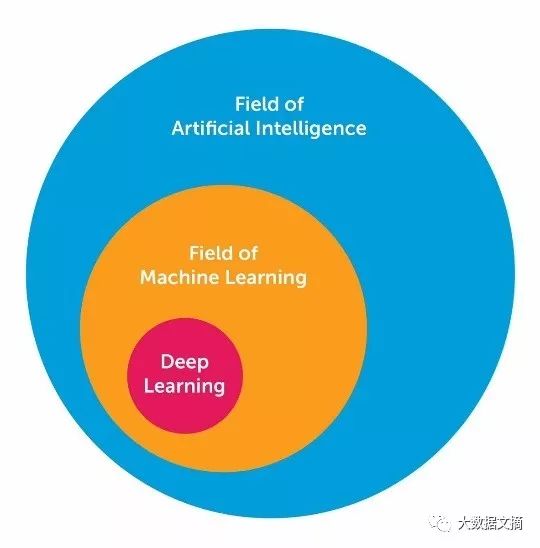
The field of artificial intelligence is broad and has been around for a long time. Deep learning is a subset of the field of machine learning, while machine learning is a subset of the AI field. Deep learning networks are generally distinguished from “typical” feedforward multilayer networks in the following aspects:
-
Deep learning has more neurons than feedforward networks
-
The connections between layers in deep learning are more complex than in feedforward networks
-
Training deep learning requires computational power similar to that of the “Cambrian Explosion”
-
Deep learning can automatically extract features
The aforementioned “more neurons” refers to the increasing number of neurons in recent years, allowing deep learning to represent more complex models. The layers have evolved from fully connected layers in multilayer networks to local connections of neuron segments in convolutional neural networks, as well as recurrent connections in recurrent neural networks (excluding connections to the previous layer).
In the four basic network architectures, deep learning can be defined as neural networks with a large number of parameters and layers:
-
Unsupervised Pre-trained Networks
-
Convolutional Neural Networks
-
Recurrent Neural Networks
-
Recursive Neural Networks
This article mainly focuses on the last three network architectures. Convolutional Neural Networks are essentially standard neural networks that extend space using shared weights. CNN recognizes images by performing convolution internally, allowing it to see the edges of objects in the image. Recurrent Neural Networks are standard neural networks that extend space using temporal extensions, extracting edges that enter the next time step rather than the same time entering the next layer. RNNs perform sequence recognition, such as speech or text signals, due to their internal cycles, meaning that short-term memory exists within RNN networks. Recursive Neural Networks are more akin to hierarchical networks, where the input sequence is actually independent of time but must be processed hierarchically in a tree-like manner. The following 10 methods apply to all of the above network architectures.
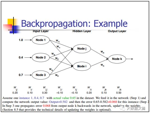
1. Back-Propagation
Back-propagation is a method for calculating the partial derivative (or gradient) of a function in a simple way, in the form of a function composition (such as a neural network). When you use gradient-based methods to solve optimization problems (gradient descent is just one of them), you want to compute the function gradient in each iteration.
For a neural network, its objective function is in composite form. How to compute the gradient? There are two conventional methods:
-
Analytical Differentiation
The function form is known, and you only need to calculate the derivative using the chain rule (basic calculus).
-
Finite Difference Approximation
This method is computationally expensive because the number of function evaluations is O(N), where N is the number of parameters. Compared to analytical differentiation, this method is much more costly. However, finite differences are often used to validate the execution of back-propagation during debugging.
2. Stochastic Gradient Descent
An intuitive way to understand gradient descent is to imagine the path of a river originating from the top of a mountain. The goal of gradient descent is precisely the goal that the river strives to achieve—flowing from the top of the mountain to the bottom (at the foot of the mountain).
Now, if the mountain’s terrain has a shape such that the river will not stop before reaching its final destination (the lowest point at the foot of the mountain), this is also the ideal situation we hope for. In machine learning, this means starting from the initial point (the top of the mountain), we have found the global minimum (or optimal value). However, due to the nature of the terrain, the river’s path may encounter several pits, causing it to get stuck and stagnate. In machine learning, these pits are known as local optima, which we do not want. Of course, there are many ways to address the local optimum issue, which I will not discuss further here.
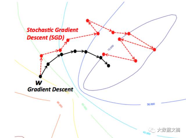
Therefore, due to the nature of the terrain (or the nature of the function in machine learning), gradient descent can easily get stuck in local minima. However, when you find a special mountain shape (like a bowl, which in machine learning terms is called a convex function), the algorithm can always find the optimal value. You can visualize this imaginary river. In machine learning, these special terrains (also known as convex functions) always need to be optimized. Additionally, depending on where you start from the top of the mountain (i.e., the initial value of the function), the path you take to reach the bottom of the mountain can be entirely different. Similarly, depending on the speed of the river (i.e., the learning rate or step size of the gradient descent algorithm), you may reach the destination in different ways. Whether you get stuck in or avoid a pit (local minimum) will be influenced by these two criteria.
3. Learning Rate Decay
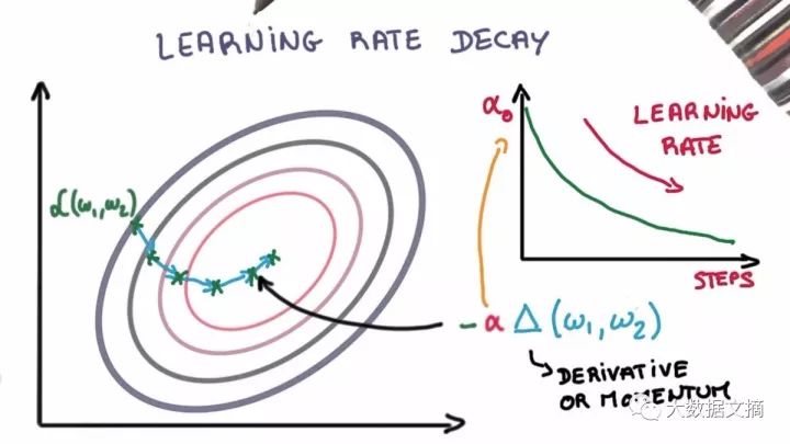
Adjusting the learning rate during the stochastic gradient descent process can enhance performance and reduce training time. This is sometimes referred to as learning rate annealing or adaptive learning rate. Gradually decreasing the learning rate over time is the simplest and most commonly used adaptive learning rate technique during training. Using a larger learning rate value in the early stages allows for significant adjustments to the learning rate; in the later stages, reducing the learning rate allows the model to update weights at a smaller rate. This technique can quickly learn some better weights in the early stages and fine-tune the weights in the later stages.
Two popular and simple learning rate decay methods are as follows:
-
Gradually reduce the learning rate at each iteration
-
At specific intervals, make a significant drop to reduce the learning rate
4. Dropout
Deep neural networks with a large number of parameters are very powerful machine learning systems. However, overfitting is a serious problem in such networks. Additionally, the slow speed of large networks makes it difficult to address the overfitting problem by combining predictions from multiple different large neural networks during the testing phase. Dropout techniques can be used to address this issue.
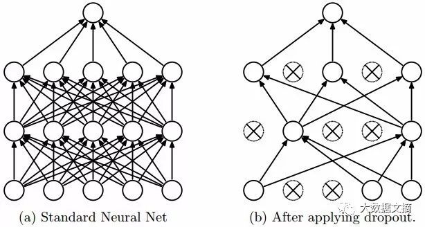
The key idea is to randomly remove units (and their corresponding connections) from the neural network during training, thereby preventing excessive adaptation between units. During training, samples are discarded in exponentially different “sparse” networks. In the testing phase, it is easy to average the predictions of these sparse networks using a single untwined network with smaller weights to approximate the result. This effectively avoids overfitting and can achieve greater performance improvements compared to other regularization methods. Dropout has been shown to enhance the performance of neural networks in supervised learning tasks across various fields, including computer vision, speech recognition, text classification, and computational biology, achieving top results in multiple benchmark datasets.
5. Max Pooling
Max pooling is a sample-based discretization method. The goal is to downsample input representations (images, output matrices from hidden layers, etc.), reduce dimensionality, and allow for assumptions about features included in sub-regions.
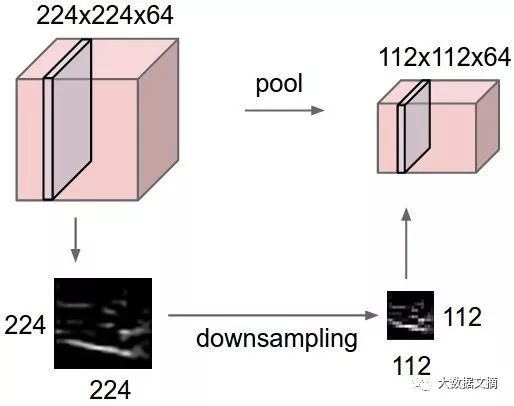
This method helps address overfitting to some extent by providing an abstract form of representation. It also reduces computational load by decreasing the number of learning parameters and providing basic internal representation invariance under transformation. Max pooling is achieved by applying a max filter to typically non-overlapping initial representation sub-regions.
6. Batch Normalization
Of course, neural networks, including deep networks, require careful tuning of weight initialization and learning parameters. Batch normalization simplifies this process.
Weight Issues:
-
Regardless of the weight initialization method, whether random or heuristically chosen, these weight values can differ significantly from the learned weights. Consider a small batch dataset; initially, there may be many outliers for the desired feature activations.
-
Deep neural networks are inherently ill-posed, meaning that small variations in the initial layers can lead to significant changes in the next layers.
During the back-propagation process, these phenomena can cause gradient shifts, meaning that before learning weights to produce the desired output, the gradients must compensate for the outliers. This results in additional time required for convergence.
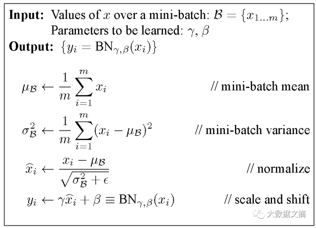
Batch normalization normalizes these gradients from discrete to normal values, allowing them to flow towards a common goal within small batch ranges (through normalization).
Learning Rate Issues:
Generally, the learning rate is kept low, allowing only a small portion of the gradients to correct the weights, as the gradients from outlier activations should not affect the already learned weights. By using batch normalization, the likelihood of these outlier activations is reduced, allowing for larger learning rates to accelerate the learning process.
7. Long Short-Term Memory (LSTM)
Long Short-Term Memory (LSTM) networks differ from neurons commonly used in other recurrent neural networks in the following three aspects:
-
It has the authority over the input to the neuron;
-
It has the authority over the storage of computed content from the previous time step;
-
It has the authority over the timing of passing output to the next time step.
The strength of LSTM lies in its ability to determine all of the above values based solely on the current input. Please see the chart below:
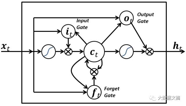
The input signal x(t) at the current time mark determines all three points above. The input gate determines the first point, the forget gate determines the second point, and the output gate determines the third point. All three decisions can be made based solely on the input. This is inspired by the brain’s mechanism, which can process sudden contextual switches based on input.
8. Skip-gram
The goal of word embedding models is to learn a high-dimensional dense representation for each vocabulary item, where the similarity between embedding vectors reflects the semantic or syntactic similarity between the corresponding words. Skip-gram is a model for learning word embeddings.
The main idea behind the skip-gram model (and many other word embedding models) is that if two vocabulary items have similar contexts, they are similar.
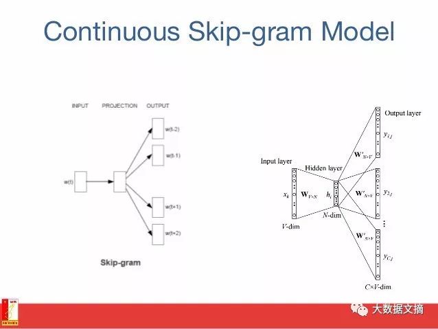
In other words, suppose you have a sentence like “cats are mammals”; if you replace “cats” with “dogs,” the sentence still makes sense. Thus, in this example, “dogs” and “cats” have similar contexts (i.e., “are mammals”).
Based on the above assumption, we can consider a context window (a window containing K continuous items). You should skip one of the words and try to learn a neural network that can predict the skipped word outside of the skipped word. Therefore, if two words repeatedly share similar contexts in a large corpus, their embedding vectors will have similar vectors.
9. Continuous Bag of Words
In natural language processing, we want to learn to represent each word in a document as a numerical vector, such that words that appear in similar contexts have very similar or close vectors. In the Continuous Bag of Words model, our goal is to use the context surrounding a specific word to predict that specific word.
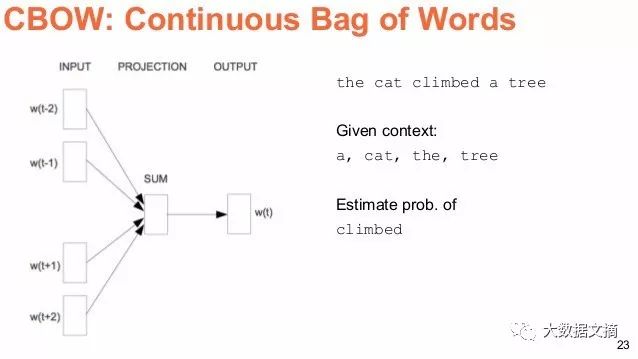
We achieve this by extracting a large number of sentences from a large corpus; each time we see a word, we simultaneously extract its context. We then input the context words into a neural network and predict the word at the center of this context.
When we have thousands of such context words and center words, we have an instance of a neural network dataset. We train this neural network, and in the final output of the encoded hidden layer, we obtain an embedded representation of the specific word. When we train on a large number of sentences, we also find that words in similar contexts happen to receive similar vectors.
10. Transfer Learning
Let’s consider how an image flows through a convolutional neural network. Suppose you have an image, apply convolution to it, and get a combination of pixels as output. Assume these outputs are edges; if you apply convolution again, the output will now be a combination of edges or lines. Then apply convolution again, and the output will be a combination of lines, and so on… You can think of it as searching for a specific pattern at each layer. The last layer of a neural network often becomes very specialized. If you train the neural network based on ImageNet, the last layer of the neural network is probably looking for overall patterns like children, dogs, or airplanes. Going back a few layers, you might see the network looking for components like eyes, ears, mouths, or wheels.
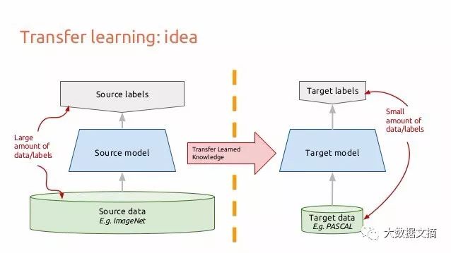
Each layer in a deep convolutional neural network gradually builds up increasingly higher-level feature representations, with the last few layers often tailored to any data at the model input end. On the other hand, the earlier layers are more generic, finding many simple patterns within a large category of images.
Transfer learning occurs when you train a CNN on one dataset, cut off the last layer, and retrain the last layer of the model on a different dataset. Intuitively, you are retraining the model to recognize different high-level features. As a result, training time is significantly reduced, so when you do not have enough data or when training requires too many resources, transfer learning is a useful tool.
This article briefly introduces some methods of deep learning. If you want to learn more and delve deeper, I recommend continuing to read the following materials:
Andrew Beam’s “Deep Learning 101” :
http://beamandrew.github.io/deeplearning/2017/02/23/deep_learning_101_part1.html
Andrey Kurenkov’s “A Brief History of Neural Nets and Deep Learning”:
http://www.andreykurenkov.com/writing/a-brief-history-of-neural-nets-and-deep-learning/
Adit Deshpande’s “A Beginner’s Guide to Understanding Convolutional Neural Networks”:
https://adeshpande3.github.io/adeshpande3.github.io/A-Beginner%27s-Guide-To-Understanding-Convolutional-Neural-Networks/
Chris Olah’s “Understanding LSTM Networks”:
http://colah.github.io/posts/2015-08-Understanding-LSTMs/
Algobean’s “Artificial Neural Networks”:
https://algobeans.com/2016/03/13/how-do-computers-recognise-handwriting-using-artificial-neural-networks/
Andrej Karpathy’s “The Unreasonable Effectiveness of Recurrent Neural Networks”:
http://karpathy.github.io/2015/05/21/rnn-effectiveness/
Deep learning is very practice-oriented. This article does not provide too many specific explanations for each new idea; most new ideas are accompanied by experimental results to demonstrate that they work. Learning deep learning is like playing with Legos; mastering Lego and other arts is equally challenging, but getting started with Lego is relatively easier.
Original link: https://towardsdatascience.com/the-10-deep-learning-methods-ai-practitioners-need-to-apply-885259f402c1
Editor: Wenjing