1. Calling Methods X=FFT(x); X=FFT(x, N); x=IFFT(X); x=IFFT(X, N) When performing spectral analysis with MATLAB, note: (1) The data structure of the return value from the FFT function is symmetric. Example: N=8; n=0:N-1; xn=[4 3 2 6 7 8 9 0]; Xk=fft(xn)
→Xk =39.0000
-10.7782 + 6.2929i
0 – 5.0000i
4.7782 – 7.7071i
5.0000
4.7782 + 7.7071i
0 + 5.0000i -10.7782 – 6.2929i Xk has the same dimensions as xn, with a total of 8 elements. The first number of Xk corresponds to the DC component, which has a frequency value of 0. (2) When performing FFT analysis, the magnitude is related to the number of points chosen for FFT, but it does not affect the analysis result. In IFFT, processing has already been done. To obtain the true amplitude value, simply multiply the result obtained after transformation by 2 divided by N.
2. Examples of FFT Applications Example 1: x=0.5*sin(2*pi*15*t)+2*sin(2*pi*40*t). Sampling frequency fs=100Hz, plot amplitude-frequency diagrams with N=128 and 1024 points. clf; fs=100; N=128; % Sampling frequency and number of data points n=0:N-1; t=n/fs; % Time series x=0.5*sin(2*pi*15*t)+2*sin(2*pi*40*t); % Signal y=fft(x,N); % Perform Fast Fourier Transform on the signal mag=abs(y); % Obtain the amplitude after Fourier transform f=n*fs/N; % Frequency sequence subplot(2,2,1), plot(f, mag); % Plot amplitude varying with frequency xlabel(‘Frequency/Hz’); ylabel(‘Amplitude’); title(‘N=128’); grid on; subplot(2,2,2), plot(f(1:N/2), mag(1:N/2)); % Plot amplitude varying with frequency before Nyquist frequency xlabel(‘Frequency/Hz’); ylabel(‘Amplitude’); title(‘N=128’); grid on;% Process signal sampling data for 1024 points fs=100; N=1024; n=0:N-1; t=n/fs; x=0.5*sin(2*pi*15*t)+2*sin(2*pi*40*t); % Signal y=fft(x,N); % Perform Fast Fourier Transform on the signal mag=abs(y); % Obtain the amplitude after Fourier transform f=n*fs/N; subplot(2,2,3), plot(f, mag); % Plot amplitude varying with frequency xlabel(‘Frequency/Hz’); ylabel(‘Amplitude’); title(‘N=1024’); grid on; subplot(2,2,4) plot(f(1:N/2), mag(1:N/2)); % Plot amplitude varying with frequency before Nyquist frequency xlabel(‘Frequency/Hz’); ylabel(‘Amplitude’); title(‘N=1024’); grid on; Running result: 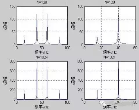 fs=100Hz, Nyquist frequency is fs/2=50Hz. The entire frequency spectrum is symmetric about the Nyquist frequency. It is also clear that the signal contains two frequency components: 15Hz and 40Hz. This illustrates the symmetry of the FFT transformed data. Therefore, when performing spectral analysis on signals using FFT, it is only necessary to examine the frequency characteristics within the range of 0 to Nyquist frequency. If the sampling frequency and sampling interval are not given, the analysis is usually normalized to frequency 0 to 1. In addition, the magnitude of the amplitude is related to the number of sampling points used; the amplitude at the same frequency using 128 points and 1024 points will show different values, but in the same graph, the amplitude ratio between 40Hz and 15Hz is 4:1, consistent with the real amplitudes of 0.5:2. To correspond to the real amplitude, the result after transformation needs to be multiplied by 2 divided by N. Example 2: x=0.5*sin(2*pi*15*t)+2*sin(2*pi*40*t), fs=100Hz, plot: (1) Number of data N=32, number of sampling points for FFT NFFT=32; (2) N=32, NFFT=128; (3) N=136, NFFT=128; (4) N=136, NFFT=512. clf; fs=100; % Sampling frequency Ndata=32; % Data length N=32; % Length of T’s data n=0:Ndata-1; t=n/fs; % Time series corresponding to the data x=0.5*sin(2*pi*15*t)+2*sin(2*pi*40*t); % Time domain signal y=fft(x,N); % Fourier transform of the signal mag=abs(y); % Obtain amplitude f=(0:N-1)*fs/N; % True frequency subplot(2,2,1), plot(f(1:N/2), mag(1:N/2)*2/N); % Plot amplitude before Nyquist frequency xlabel(‘Frequency/Hz’); ylabel(‘Amplitude’); title(‘Ndata=32 Nfft=32’); grid on; Ndata=32; % Number of data N=128; % Length of data used n=0:Ndata-1; t=n/fs; % Time series x=0.5*sin(2*pi*15*t)+2*sin(2*pi*40*t); y=fft(x,N); mag=abs(y); f=(0:N-1)*fs/N; % True frequency subplot(2,2,2), plot(f(1:N/2), mag(1:N/2)*2/N); % Plot amplitude before Nyquist frequency xlabel(‘Frequency/Hz’); ylabel(‘Amplitude’); title(‘Ndata=32 Nfft=128’); grid on; Ndata=136; % Number of data N=128; % Length of data used n=0:Ndata-1; t=n/fs; % Time series x=0.5*sin(2*pi*15*t)+2*sin(2*pi*40*t); y=fft(x,N); mag=abs(y); f=(0:N-1)*fs/N; % True frequency subplot(2,2,3), plot(f(1:N/2), mag(1:N/2)*2/N); % Plot amplitude before Nyquist frequency xlabel(‘Frequency/Hz’); ylabel(‘Amplitude’); title(‘Ndata=136 Nfft=128’); grid on; Ndata=136; % Number of data N=512; % Length of data used n=0:Ndata-1; t=n/fs; % Time series x=0.5*sin(2*pi*15*t)+2*sin(2*pi*40*t); y=fft(x,N); mag=abs(y); f=(0:N-1)*fs/N; % True frequency subplot(2,2,4), plot(f(1:N/2), mag(1:N/2)*2/N); % Plot amplitude before Nyquist frequency xlabel(‘Frequency/Hz’); ylabel(‘Amplitude’); title(‘Ndata=136 Nfft=512’); grid on;
 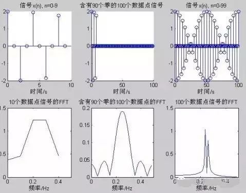 Conclusion: (1) When both the number of data points and the number of data points used for FFT are 32, the frequency resolution is low, but there are no other frequency components caused by zero-padding. (2) Due to adding zeros in the time domain signal, many other components appear in the amplitude spectrum, which is caused by zero-padding. The amplitude is significantly reduced due to the addition of multiple zeros. (3) The FFT program truncates the data, resulting in higher resolution. (4) Also, zero-padding at the end of the data, but since the number of data points containing the signal is sufficient, the FFT amplitude spectrum is basically unaffected. When performing frequency spectrum analysis on signals, the data samples should have sufficient length; generally, the number of data points used in the FFT program should be the same as the original signal data points, so that the frequency spectrum plot has high quality and can reduce the effects caused by zero-padding or truncation. Example 3: x=cos(2*pi*0.24*n)+cos(2*pi*0.26*n)

(1) Too few data points make it almost impossible to see detailed information about the signal spectrum; (2) The middle graph shows x(n) padded with 90 zeros, resulting in a very dense amplitude frequency spectrum, known as a high-density spectrum. However, it is difficult to see the frequency components of the signal from the graph. (3) With a long effective data length, the frequency components of the signal can be clearly observed; one is 0.24Hz and the other is 0.26Hz, known as a high-resolution spectrum. It can be seen that when sampling data is too few, using FFT transformation cannot distinguish the frequency components. Adding zeros increases the number of data points in the spectrum, enhancing the density of the spectrum, but still cannot distinguish the frequency components, meaning the resolution of the spectrum has not improved. Only when the number of data points is sufficient can the frequency components be distinguished.