Understanding SIMD in Computer Architecture

1. Introduction

In previous articles, we explored the concepts related to Instruction Level Parallelism (ILP). Clearly, in addition to instruction-level parallelism, processors also exhibit parallelism in other dimensions. This article presents the SIMD technology within Data Level Parallelism (DLP). First, let’s consider a question: why was data-level parallelism developed? Does relying solely on ILP have drawbacks?

Let’s review the basic concept of ILP. ILP refers to executing multiple instructions simultaneously within a single processor, typically including techniques like pipelining, VLIW, and out-of-order superscalar technology. Due to the dominance of out-of-order superscalar technology in general CPUs, ILP is often assumed to refer to out-of-order superscalar processors. These techniques are undoubtedly effective, significantly improving IPC and thus enhancing performance. However, ILP does not fully exploit the parallelism inherent in applications.

We might think of ILP as essentially running more instructions in one cycle. It has significant advantages in general processing, as any program will be compiled into a series of instructions. From the perspective of executing more instructions per cycle, this is indeed a very good solution paradigm.

But this raises a new question: are these instructions generated by the program really optimal? Do certain applications genuinely require many instructions to complete? Is it possible that the application itself contains inherent parallelism? Could a code segment that originally required a dozen or so instructions be completed with just a couple of instructions through special hardware architecture combined with instruction encoding? The answer is certainly yes; DLP is one of the solutions to this problem. Besides the insufficient extraction of inherent parallelism in programs (as ILP does not actually utilize the parallelism present in the program itself), ILP also has the following drawbacks:

• With the limitations of process technology, the benefits brought by Moore’s Law are no longer available, and clock frequency can no longer be continuously improved;

• Increasing pipeline stages to enhance clock frequency has led to the “high frequency, low energy” problem (branches, hazards);

• In scenarios like scientific computing and streaming media processing, due to poor locality, cache hit rates have declined;

As scientific computing, video processing, and emerging machine learning applications have become more widespread, it has gradually been recognized that these algorithms often naturally exhibit data parallelism. Thus, the concept of DLP has evolved, which was popularized in the 1970s by American electrical engineer Seymour Cray, who introduced a series of scientific computing processors based on DLP ideas, such as CRAY-1 and CRAY-2. Here, we introduce our topic DLP through a quote from Mr. Cray.

2. SIMD Architecture

Typical DLP technologies include vector processors, SIMD, and GPUs. Vector processors and SIMD are quite similar, and GPUs are merely a variant of SIMD. Once you master SIMD, it becomes much simpler to grasp other DLP technologies, so this article focuses on SIMD.

2.1 Flynn’s Taxonomy

In 1966, American computer scientist Michael J. Flynn proposed the concept of “Flynn’s taxonomy.” Although this classification may not be very accurate by today’s standards, it still allows us to categorize computers roughly in a short time.

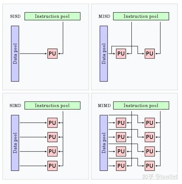
Flynn classified computers into four major categories based on whether instructions and data are parallel:

• SISD: Single Instruction Single Data, most low-end MCUs are of this type, such as Cortex-M0/3;

• SIMD: Single Instruction manipulating multiple data elements, including Array processors and Vector Processors;

• MISD: Multiple Instructions controlling a single data stream, which is very rare, somewhat similar to a 1-D pulsed array;

• MIMD: Multiple Instructions controlling multiple data elements, very common in supercomputers, and multi-threaded processors are MIMD architectures;

2.2 Differences Between SIMD and MIMD

Let’s briefly compare SIMD and MIMD; both are parallel data streams, but where do their differences lie?

For MIMD, its core idea is that multiple instructions control multiple data streams, and these multiple instruction streams can be completely independent, making it very useful for applications that require simultaneous execution of multiple different operations, such as distributed computing. Additionally, MIMD typically has higher flexibility because each processing unit can independently execute different instructions.

Of course, MIMD cannot be perfect in every aspect, and it must have drawbacks for other models to exist (whether in engineering or research, you must propose something new because another thing has its shortcomings; if everything is perfect, there’s no need for a new solution). Let’s consider what drawbacks MIMD has:

First, its high flexibility inevitably leads to increased design complexity, thus “rules represent simplicity.” MIMD needs to manage multiple independent instruction streams and data streams, making programming and scheduling very complex, which is difficult for software developers. In contrast, SIMD allows programmers to adopt a sequential thinking approach while achieving parallel speedup (the architecture bible refers to this as SIMD’s greatest advantage over MIMD). Additionally, MIMD has issues such as synchronization and communication overhead, and resource utilization. Despite these drawbacks, MIMD remains very effective in many parallel computing scenarios, and these issues can be overcome through reasonable design and optimization; we will discuss these topics later. Let’s continue to focus on SIMD.

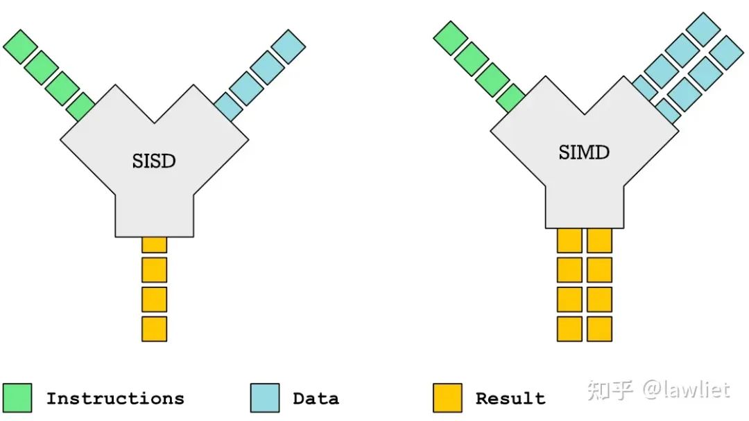
I believe SIMD has two main advantages over MIMD: one is that it is more energy-efficient than MIMD, as it only requires fetching instructions once for each group of data operations, especially in scenarios like PMD (Personal Mobile Devices) where power consumption is critical, SIMD is very useful. Moreover, as mentioned earlier, SIMD allows programmers to adopt a sequential thinking approach while achieving parallel speedup. Anyone with experience in parallel programming knows that writing parallel programs is very challenging, with issues like contention and deadlocks. There are many considerations, whereas SIMD simplifies this as you are executing just one instruction.

2.3 Vector Processors

When discussing SIMD, one cannot avoid vector processors. Many people are very picky about the distinction between these two concepts, which I believe is unnecessary to differentiate too clearly. One can simply understand that SIMD is a design philosophy for computer architecture, while vector processors are the specific hardware implementations of SIMD computation. A vector processor is a processor that supports a SIMD instruction set for executing parallel vector computation tasks.

Of course, many processors are not just vector processors, as they can generally run scalar operations as well as execute vector operations. In addition to so-called vector processors, SIMD instruction extensions on general processors and GPUs can also implement SIMD mechanisms.

The term vector is relative to scalar, representing a set of data. Many specific programs actually operate on vectors. For example, the following is a very typical vector operation (remember this example, as it will be used later).

for (i = 0; i <= 49; i++)
    C[i] = (A[i] + B[i]) / 2

Vector processors operate on vectors rather than scalars, and they typically have the following basic mechanisms:

• Need to Load/Store vectors, hence vector registers are required;

• Need to operate on vectors of different lengths for flexibility, thus a Vector Length Register (VLEN register) is necessary;

• Additionally, vector data may exist at different memory locations, necessitating a Vector Stride Register (VSTR register);

• Stride refers to the distance between two adjacent elements in a group of vectors in memory;

Let’s look at an example of Vector Stride, which is very common in multimedia processing and AI computations: matrix multiplication.

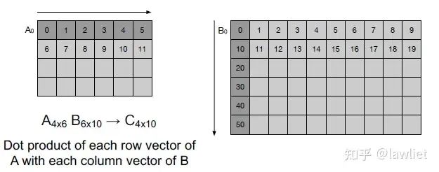
Assuming we have matrices A and B stored in memory in row-major order, as shown below. If there is no Stride, we would multiply the rows of A with the rows of B, which obviously does not comply with the rules of matrix multiplication. At this point, we need the VSTR register, configured as follows:

• Load Row0 of A (A0 to A5) into vector register V1;

• Each time, only increment the address by 1 to fetch the next column data;

• Stride is 1;

• Load Column0 of B (B0 to B50) into vector register V2;

• Each time, increment the address by 10 to fetch the next row data;

• Stride is 10;

For vector processors, each consecutive cycle processes data elements, so:

• Vector functional units are pipelined;

• Each level of the pipeline operates on different data elements;

Let’s look at the following diagram; what are the benefits of vector-based operations? Assuming we are still using a superscalar processor, wouldn’t it also achieve parallelism by executing multiple instructions simultaneously? Clearly, a superscalar processor executing a series of additions continuously will encounter data hazards and structural hazards. In contrast, the structured design of vector processors naturally avoids these problems. You can see that a series of additions can be computed without issue. Moreover, the elements within these vectors are independent, allowing for deeper pipelining, since there’s no need to consider conflict issues, thus further increasing the clock frequency. Additionally, due to the presence of Stride, the addresses of vector elements are straightforward, facilitating easy data loading (including prefetching operations, etc.);

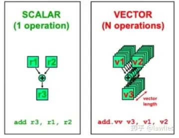
With all these advantages, what are the drawbacks of vector processors? You may have already noticed that so far, the data we’ve operated on has been very regular vectors, and when the parallelism is irregular, vector processors can become very inefficient. For example, searching for a key in a linked list, you can imagine how a vector processor would handle this; in reality, it would be akin to a scalar processor, wasting a lot of components. This drawback is similar to VLIW; when there aren’t enough parallel operations, efficiency will naturally decline.

Let’s consider where the performance bottleneck of vector processors lies. Since vector processors need to operate on so many data elements simultaneously, if these data require many cycles to retrieve, it could lead to computational units being idle, thereby affecting performance. The most typical performance bottleneck of vector processors is Memory (Bandwidth). This is particularly true in the following situations:

1. When the ratio of computation to memory operations is not well controlled (e.g., when the actual computation is minimal and memory operations are excessive);

2. Data is not distributed across multiple Memory Banks (more details later);

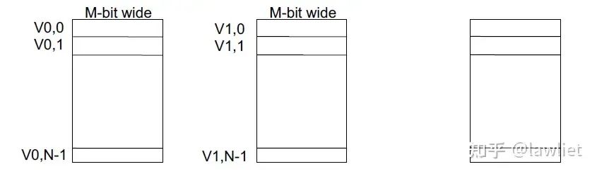
Let’s take a look at vector registers. For each vector register, there are N groups, each group being M bits; additionally, vector control registers include: VLEN, VSTR, VMASK; where VLEN cannot exceed N, as previously mentioned.

As for what VMASK is: the VMASK register is usually a bit vector, where each bit corresponds to an element in the vector. If the corresponding bit is 1, it indicates that the element participates in the vector operation; if the bit is 0, it indicates that the element is masked or ignored. By using the VMASK register, selective processing or filtering of elements during vector operations can be achieved.

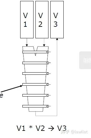
As mentioned earlier, due to the independence of elements within vectors, vector processors are naturally suited for deep pipelining, as it is easy to control. The following diagram illustrates a six-stage pipelined multiplier.

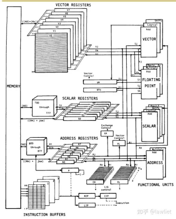
When mentioning vector processors, one cannot forget CRAY, which produced early supercomputers, and in that era, supercomputers were synonymous with vector machines. The most famous of these is the CRAY-1, launched in 1978, whose architecture is illustrated below:

• Has vector and scalar modes;

• 8 vector registers with 64 elements (maximum parallelism of 64);

• Each element is 64 bits;

• 16 Memory Banks;

8 scalar registers of 64 bits;

• 6 address registers of 24 bits;

Most of these elements are likely easy to understand. However, what does the 16 memory banks mean?

As discussed earlier, loading and storing vectors is inherently more complex than scalar processors, as it needs to load/store multiple elements. The elements are spaced at fixed distances (Stride).

Assuming a Stride of 1, we continuously load elements into our registers, theoretically, we can load one element per cycle. But what if accessing Memory takes more than one cycle? If the previous data hasn’t returned yet, and a new address is issued, Memory theoretically does not support such pipelined operations (ordinary RAM lacks an Outstanding mechanism).

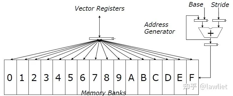
The answer is to divide Memory into chunks, creating multiple BANKs and interleaving elements across different BANKs!

By dividing into multiple BANKs, there are several advantages. BANKs are smaller, thus reducing the corresponding MUX logic, and SRAM output delay decreases, potentially eliminating the need for multiple cycles. Additionally, clearly, multiple BANKs can theoretically achieve N levels of parallelism, as each BANK is independent and can be accessed in parallel. Even if multiple cycles are still needed to return data, multiple BANKs can at least guarantee a throughput of one element per cycle, which we will see how it is implemented.

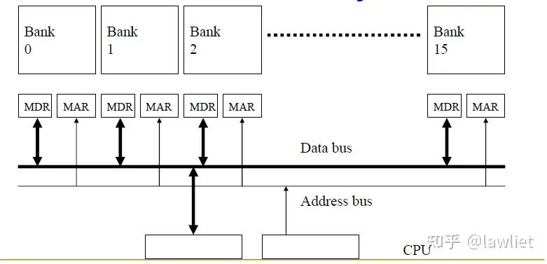
Let’s look at the diagram below. Assuming each element is interleaved between BANKs and the Stride equals 1, and the number of BANKs exceeds the Access Latency! In this case, we can ensure that at least one element is obtained per cycle without introducing extra overhead. For instance, in the following diagram, if it takes 16 cycles to return data, the master side simply needs to provide addresses normally. After 16 cycles, the data from BANK 0 returns, and after 17 cycles, the data from the first BANK returns, and so on. This way, we achieve what is known as Outstanding, while the BANK return cycles are fixed, ensuring the order (this type of RAM is usually private RAM, and other modules should not use it; otherwise, the data return order will be disrupted).

Let’s return to the earlier C code example. How many clock cycles would it take if we implemented it in scalar code?

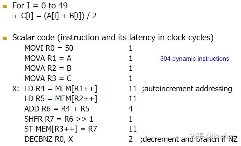
The corresponding assembly code is shown above, with the numbers indicating how many cycles are needed. Assuming we are running on a scalar execution sequential processor with only one Memory BANK.

• The LOAD operation cannot be pipelined (as explained earlier), requiring 2*11=22 cycles, so the loop body takes 40 cycles;

• The total operation runs for 4+50 (loop 50 times)*40+4=2004 cycles;

Now let’s assume our Memory has two read/write ports, i.e., true dual-port RAM, or a 2-BANK Memory. How many cycles would it take then? In this case, two LOADs can operate in a pipelined manner, thus the loop body only requires 11+1+4+1+11+2=30 cycles, leading to a total of 4+50*30=1504 cycles, immediately reducing by 500 cycles! This demonstrates that multiple BANKs provide significant optimization for vector operations.

Now, let’s assume we are running on a vector processor with 16 Memory BANKs. How many cycles would it take?

For the vector processor, this example would not involve a loop; the corresponding assembly code is as follows:

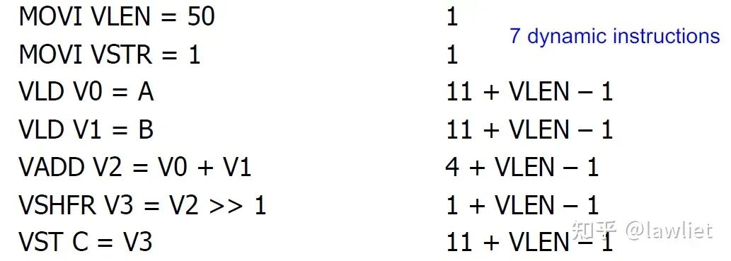
How many cycles would this take?

Actually, it’s the sum of the cycles above; since VLEN=50, it requires a total of 285 cycles.

Now, let’s consider why we need 16 BANKs. Since the Memory Access delay is 11 cycles, we need more than 11 BANKs, and BANKs are generally powers of two, so we choose 16. In the example above, we assumed a Stride of 1, which is fine, but what if the Stride is greater than 1? For instance, if the Stride is 16, we would be accessing the same BANK every time, effectively doing useless work. Thus, for scenarios where the Stride exceeds 1, we need to think of further solutions.

Let’s consider if further optimization is possible. The answer is yes. Looking at the assembly code above, the VADD operation requires operands from V0 and V1. Is it possible to forward them directly during LOAD to the multiplier? Yes! In vector processors, this is generally not called Forwarding; it’s referred to as Vector Chaining, as illustrated in the diagram below.

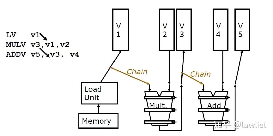
Using this technique, we can accelerate the initial computation. The initial computation took 285 cycles, as shown in the diagram below:

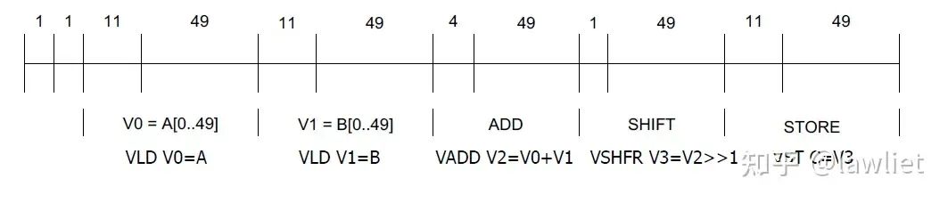
However, we can route the VLD directly to the VADD. Let’s consider expanding the BANK to have two read and one write. This way, we can perform VLD operations in parallel. Once the first data returns, instead of storing it back to the vector register, we directly send it to the adder for computation. This method only requires 79 cycles, achieving a performance improvement of 19 times compared to the original scalar processor’s 2004 cycles!

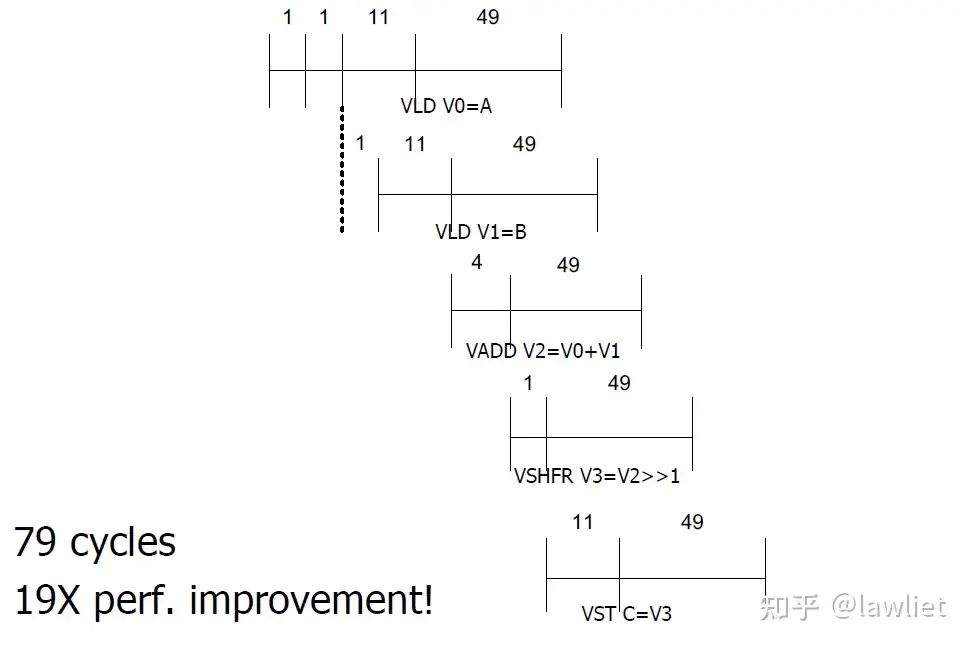
Let’s summarize the ideas above:

• Utilize the inherent parallelism in programs; two groups of vectors can be loaded in parallel, even LOAD+STORE (by expanding BANK to two read ports);

• Data is already available, so there’s no need to store it back to registers. Directly send it to the computational unit for processing; (Forwarding concept)

Now, let’s consider what to do if the number of data elements exceeds the number of elements that can be stored in the vector register. It’s simple; if it can’t be calculated in one go, just divide it into multiple calculations. For example, if there are 527 elements, and the vector register can only hold 64 elements (the maximum parallelism is 64), it can be computed in 8 iterations. This method is known as Vector Stripmining.

2.4 SIMD Operations in ISA

In addition to dedicated vector processors, many general processors have also added SIMD-related instruction set extensions, allowing us to experience SIMD mechanisms even on general processors.

For SIMD instruction set extensions, the following characteristics are typically observed:

• A single instruction operates on multiple data sets at once (the characteristic of SIMD);

• Commonly used in graphics operations, multimedia computations, machine learning, etc.;

• Executes short arithmetic operations (also referred to as packed arithmetic).

Let’s look at the example below, adding 4 sets of 8-bit data. Without vector instruction extensions, it would require 4 addition operations, not to mention data hazards and structural hazards. However, with vector instruction extensions, it can be done in one cycle.

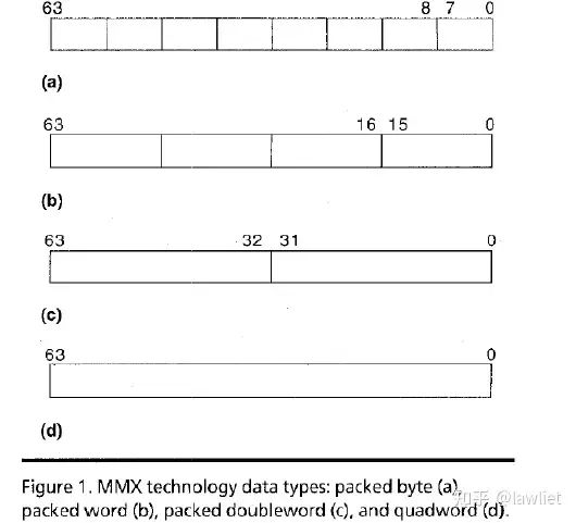
When discussing SIMD instruction extensions, one must mention Intel’s related instructions, the most famous of which is Intel’s MMX operations, which were first introduced in its Pentium series processors. The core idea is to operate on multiple data elements simultaneously, i.e., the SIMD concept. For 64-bit processors, it can be split into 8 8-bit, 4 16-bit, 2 32-bit, or 1 64-bit, and then the corresponding operations can be performed. The idea is straightforward and is not fundamentally different from the SIMD examples I will mention later.

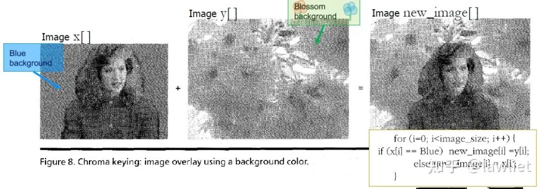
This instruction extension was initially used in image processing. Let’s look at an example of image overlay.

The so-called image overlay means combining two images. The mechanism for the overlay is that for the Blue background image, it uses Image Y; otherwise, it uses Image X. This example involves a large number of parallel computations. In fact, there are no dependencies between the individual PIXELS, allowing for parallel computations, making this algorithm suitable for acceleration using SIMD.

MMX is an early SIMD instruction extension, and under the X86 architecture, there are the following SIMD instruction extensions:

• MMX

• SSE (Streaming SIMD Extensions)

• SSE-1

• SSE-2

• SSE-3

• SSE-4

[manim] Animation demonstration of SSE instruction set SIMD intrinsics (Part 1) _ Bilibiliwww.bilibili.com/video/BV1nX4y147aB/?spm_id_from=333.788&vd_source=aa30a4e19bdd942dc58f16b3be44358e

• AVX (Advanced Vector Extensions)
• AVX: 256-bit Float Point
• AVX2: 256-bit Float Point with FMA extension (Fused Multiply Add)
• AVX-512: 512-bit
• AMX (Advanced Matrix Extensions)
• For AI computations
• Two-dimensional registers
• Tiled matrix multiply unit (TMUL)

In addition to Intel, ARM also has corresponding SIMD instruction extensions NEON, which you can refer to the relevant documentation:https://developer.arm.com/Architectures/Neondeveloper.arm.com/Architectures/NeonAdditionally, RISC-V also has corresponding vector extensions. Below is a very good popular science article translated into Chinese; those with good English skills are recommended to read the original:Sun Kuikui: Comparison of Vector Extensions of ARM and RISC-V55 Likes · 6 Comments Article

2.5 SIMD Operations in Accelerators (Including but Not Limited to) Machine Learning

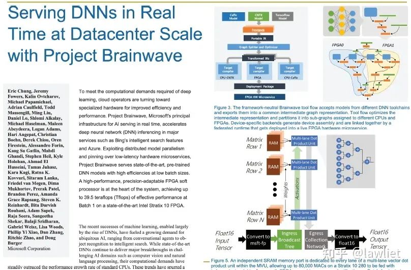
In addition to dedicated vector processors and general processor SIMD extensions, many neural network accelerators also feature SIMD mechanisms, as previously mentioned, SIMD is a concept. A concept does not necessarily have to be implemented by a specific type of processor. I do not intend to elaborate on this part; I recommend Microsoft’s Brainwave project, which has many papers available for further understanding. In summary, it’s important to know that SIMD exists in many places.

3. An Example of SIMD

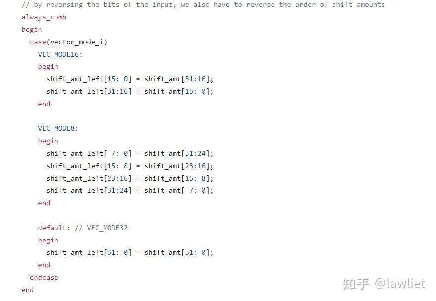
The author previously worked on instruction-level extensions, focusing on the PULP open-source project, which includes the RI5CY processor core, which looks something like this:

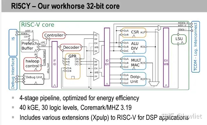
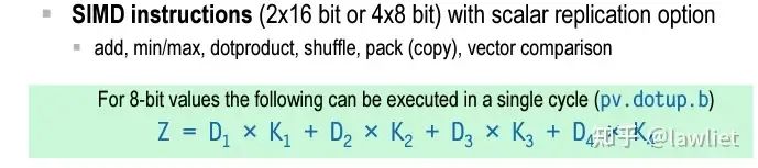
The ALU module supports SIMD operations. The code is open-source here:https://github.com/embecosm/ri5cy/blob/verilator-model/alu.svgithub.com/embecosm/ri5cy/blob/verilator-model/alu.svLet’s take a look at how it works. I’ve extracted a code snippet; the vector operations of this processor are very simple. It does not have the concept of vector registers, using ordinary registers instead, treating a 32-bit operand as two 16-bit or four 8-bit numbers for computation, and then writing back to the registers. Interested readers can check the source code.

4. Conclusion

After reading this article, you should have a clear understanding of the shortcomings of ILP and the basic concepts of SIMD. SIMD is currently widely used, with specific architectural implementations primarily concentrated in the following three architectures:

• Vector processors;
• General processors with SIMD instruction set extensions;
• GPUs and some NPUs;

This article concludes here. I hope it is helpful to everyone. Please feel free to point out any errors.