Particle Swarm Optimization Algorithm for Solving Model Parameters (Including MATLAB Code)

Particle Swarm Optimization Algorithm

※

Table of Contents

(1) Algorithm Introduction;

(2) Algorithm Process;

(3) Advantages and Disadvantages of the Algorithm and Improvements;

(4) Application Areas;

(5) MATLAB Code Example;

※

1. Algorithm Introduction

The Particle Swarm Optimization (PSO) algorithm is a type of swarm intelligence optimization algorithm proposed by Kennedy and Eberhart in 1995, inspired by the foraging behavior of birds. It is a population-based stochastic search algorithm primarily used for function optimization, machine learning, path planning, and other problems.

Basic Idea: Imagine a flock of birds searching for food in an area; they do not know the location of the food, but they can adjust their flight direction based on their current experience (personal best position) and the experiences of other birds around them (global or neighborhood best position), gradually approaching the food.

In PSO, each “bird” is abstracted as a particle, and the entire flock is a swarm of particles. Each particle represents a solution, flying in the search space to find the optimal solution.

※

2. Algorithm Process

(1) Initialization

Number of particles: N;

Position of each particle xi: represents the current solution;

Velocity of each particle vi: represents the search direction and magnitude;

Each particle records its best encountered position pi (individual extremum);

The entire swarm records the best position g (global extremum);

(2) Iterative Update Formula

For each individual (candidate solution), evaluate its quality using a fitness function. In materials science, the fitness function is often defined by comparing the error between model predictions and experimental data. For example, the Mean Squared Error (MSE) can be used to measure the prediction accuracy of the model.

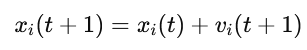
During each generation iteration, the velocity and position of each particle are updated according to the following formulas:

Velocity Update:

Position Update:

Where:

ω: Inertia weight (controls the influence of the previous velocity on the current one);

c1,c2: Learning factors (usually set to 2), controlling the weights of individual experience and group experience, respectively;

r1,r2: Random numbers between [0,1];

pi: Individual historical best position;

g: Group historical best position;

(3) Update Individual and Global Best Solutions

If the current particle position is better than its historical best position, update pi; if the current particle position is better than the global best position, update g.

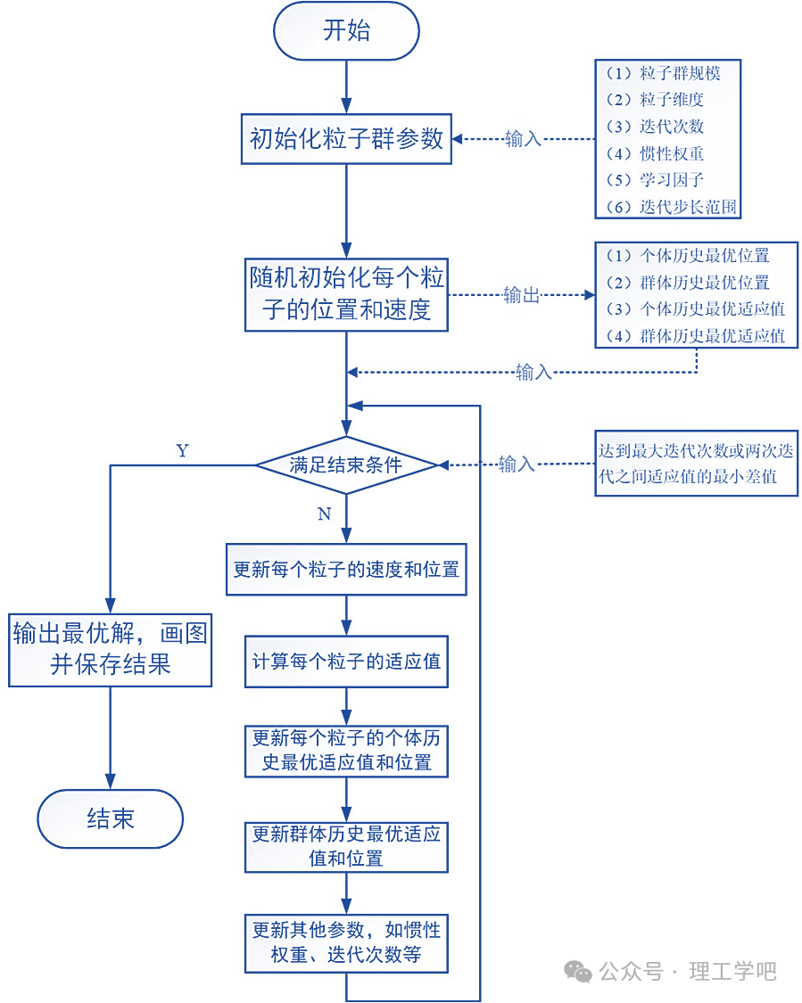
(4) Check for Termination

If the maximum number of iterations is reached or the error meets the criteria, stop; otherwise, return to step 2 to continue iterating.

※

3. Advantages and Disadvantages of the Algorithm and Improvements

Advantages: Simple implementation, few parameters; fast convergence speed, especially in the early stages; suitable for solving multi-dimensional continuous optimization problems; can be combined with other optimization algorithms (such as genetic algorithms, simulated annealing) to improve performance.

Disadvantages: Prone to getting stuck in local optima (especially in high-dimensional non-convex problems); parameters (such as inertia weight) are sensitive to performance; there is a trade-off between convergence speed and accuracy.

To overcome the above shortcomings, PSO improvements include but are not limited to:

(1) Linearly decreasing inertia weight (allowing particles to explore more in the early stages and converge quickly in the later stages);

(2) Local neighborhood models (reducing global dependence and increasing diversity);

(3) Hybrid algorithms (combining with GA, simulated annealing, etc.);

(4) Quantum Particle Swarm Optimization (using probability distributions instead of positions and velocities), etc.

※

4. Application Areas

Application areas: data mining, machine learning, engineering design optimization, energy systems, healthcare, and robotics, etc.

※

5. MATLAB Code Example

Assuming we want to minimize the function f(x,y)=x²+y², with the target minimum value being 0 (the origin).

Using PSO:

(1) Initialize 10 particles, each randomly distributed in [-10,10];

(2) Move each time according to the velocity and position update formulas;

(3) Particles gradually approach (0,0), which is the minimum of the function.

MATLAB code example (visualizing the movement of particles in the search space):

clc; clear; close all%% Parameter SettingsnParticles = 30;          % Number of particlesnIterations = 100;        % Number of iterationsdim = 2;                  % Problem dimensionxRange = [-10 10];        % Search space rangevMax = (xRange(2) - xRange(1)) * 0.2; % Maximum velocityw = 0.7;                  % Inertia weightc1 = 1.5;                 % Individual learning factorc2 = 1.5;                 % Social learning factor%% Initialize particle positions and velocitiesx = rand(nParticles, dim) * (xRange(2) - xRange(1)) + xRange(1); % Positionv = zeros(nParticles, dim); % Initial velocitypBest = x;                        % Individual bestpBestVal = sum(pBest.^2, 2);      % Objective function value[gBestVal, idx] = min(pBestVal);  % Global bestgBest = pBest(idx, :);%% Visualization background: draw contour of the objective function[X, Y] = meshgrid(xRange(1):0.5:xRange(2), xRange(1):0.5:xRange(2));Z = X.^2 + Y.^2;figurecontour(X, Y, Z, 50); hold oncolorbartitle('Particle Swarm Optimization Illustration (PSO)')xlabel('x'); ylabel('y');axis equal%% Main Loopfor iter = 1:nIterations    % Update velocity and position    r1 = rand(nParticles, dim);    r2 = rand(nParticles, dim);    v = w * v ...        + c1 * r1 .* (pBest - x) ...        + c2 * r2 .* (gBest - x);    % Limit maximum velocity    v = max(min(v, vMax), -vMax);    % Update position    x = x + v;    % Keep within search space    x = max(min(x, xRange(2)), xRange(1));    % Update individual best    fVal = sum(x.^2, 2);    update = fVal < pBestVal;    pBest(update, :) = x(update, :);    pBestVal(update) = fVal(update);    % Update global best    [newGBestVal, idx] = min(pBestVal);    if newGBestVal < gBestVal        gBestVal = newGBestVal;        gBest = pBest(idx, :);    end    % Visualize particle positions    cla;    contour(X, Y, Z, 50); hold on;    plot(x(:,1), x(:,2), 'bo', 'MarkerFaceColor', 'b'); % Particles    plot(gBest(1), gBest(2), 'r*', 'MarkerSize', 10);   % Global best    title(['Iteration: ' num2str(iter) ', Best Value: ' num2str(gBestVal, '%.4f')])    xlabel('x'); ylabel('y');    axis equal    pause(0.05);endfprintf('\nFinal Best Value: %.6f at (x, y) = (%.4f, %.4f)\n', gBestVal, gBest(1), gBest(2));

Optimization Results:

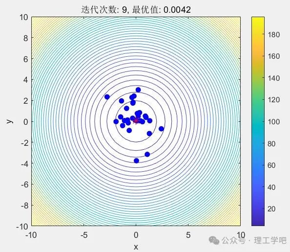
Iteration 9

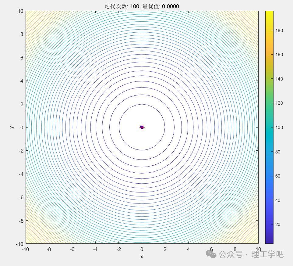
Iteration 100

Output:

Final Best Value: 0.000000 at (x, y) = (0.0000, 0.0000)

Editor: Li Donghong

Reference: MATLAB Toolbox,

Content for educational purposes only, commercial use is prohibited.