Technical Interpretation of DeepSeek (1) – A Comprehensive Understanding of MLA (Multi-Head Latent Attention)

Zhihu: Jiang Fuchun (Authorized) Link: https://zhuanlan.zhihu.com/p/16730036197 Editor: “Deep Learning Natural Language Processing” WeChat Official Account

Introduction

DeepSeek has recently gained significant attention, and I have been following some of the technical reports released by DeepSeek. They have consistently surprised everyone with their model training, inference performance, and computational costs. After reading DeepSeek’s technical reports, I have two strong impressions. First, DeepSeek is meticulous in the details of their models, having made significant modifications to some model frameworks (for example, in model optimization: MLA, GRPO, MTP); second, their engineering capabilities are indeed strong, as they can agilely integrate mainstream frameworks and technical points into their own systems (for instance, in terms of infrastructure, we can see core technologies from frameworks like DeepSpeed, Megatron, DistServer, vLLM, etc.). I plan to write a few notes to study and organize DeepSeek’s technologies.

This article focuses on explaining MLA (Multi-Head Latent Attention).

Note: During my learning process, I often encounter knowledge blind spots or areas where my understanding is not precise, so I recursively study some extended contexts. This article will also layer the necessary background knowledge to interpret the background of MLA, the problems it aims to solve, and the final effects.

MLA primarily reduces memory usage by optimizing the KV-cache, thereby improving inference performance. Presenting this conclusion directly may not be easy to understand. First, let’s look at what a complete inference phase looks like for generative models and what issues exist regarding inference performance.

All LLM subfield groups and submission groups can enter from here!

1. LLM Model Inference Process

LLM inference is divided into two stages: prefill stage and decode stage

• prefill stage: This is when the model computes all Prompt tokens in parallel at once, ultimately generating the first output token.
• decode stage: This generates one token at a time until the EOS (end-of-sequence) token is produced, resulting in the final response.

During the inference process, since the model stacks multiple layers of transformers, the core computational consumption occurs within the Transformer, including operations like MHA and FFN, where MHA calculates the Q, K, and V matrices to perform multi-head attention calculations.

In the LLM generation process, it is a process of predicting the next token based on the forward sequence of tokens, where tokens in the sequence (whether in the prefill stage or the decode stage) only interact with the preceding tokens to compute attention, which we also refer to as Causal Attention. The matrix computation is implemented through a lower triangular Causal Attention Mask, allowing token interactions to only perceive the forward sequence. As shown in Figure 1, the internal details of the Transformer are displayed:

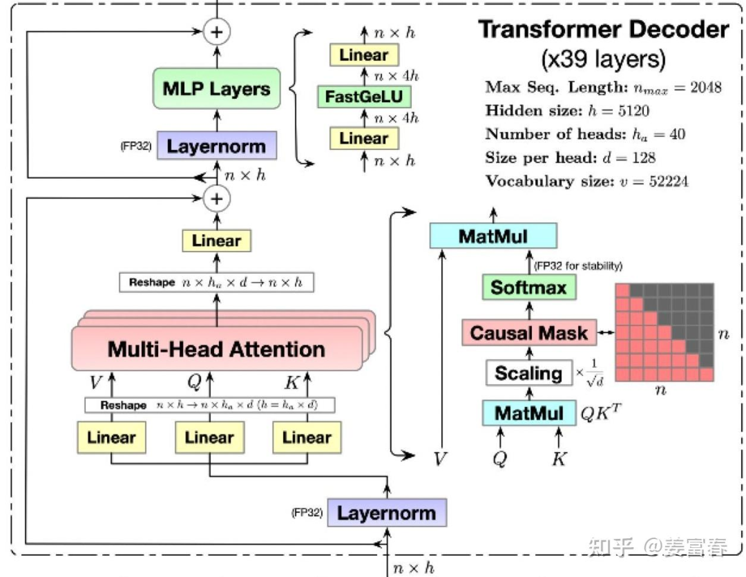
Taking a token at a position in a sequence as an example, we calculate the attention process of one layer of the Transformer, as shown in the formula below:

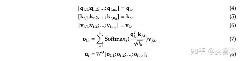
Symbols in the formula: represent the calculation of the th token in the sequence; has two subscripts, the first indicating the token position and the second indicating the corresponding Head index.

From formula (7), we can see that when calculating Attention, the th position only interacts with the preceding th position, leading us to the following two conclusions:

1. The calculation of the preceding is not influenced by subsequent tokens.
2. The attention of the th position must use the value of the preceding th position, which remains constant.

Therefore, to accelerate training and inference efficiency, during the token-by-token generation process, to avoid redundant calculations of the preceding , researchers proposed caching the previously computed , which is the current mainstream KV-cache mechanism. The essence of KV-cache is to exchange space for time. We know that current LLM sizes are relatively large, and GPU memory is also quite precious; storing KV-cache in memory will inevitably lead to memory access bottlenecks. In other words, if the model computes directly without KV-cache (repeating calculations of the preceding ), it becomes a computation-intensive task; with KV-cache, the model no longer computes but reads from the “storage medium,” leading to frequent read and write operations between the GPT core and the storage medium, thus becoming a memory access-intensive task. Therefore, while the KV-cache mechanism solves the problem of redundant calculations, the memory access rate directly affects the speed of training and inference.

Next, let’s take a closer look at the memory access rates at different levels for a typical inference architecture, what data needs to be stored during the model inference process, and how to allocate storage.

2. Memory Usage During LLM Inference Stage

2.1 Memory Access Rate Levels

To intuitively understand the memory access rates, let’s take a distributed inference architecture as an example.

For instance, with 2 machines, each having 8 A100 GPUs, the data access efficiency within the card, between single machine cards, and across machines is shown in Figure 3. Note: In our example, we only describe one type of memory medium, HBM (which we commonly refer to as GPU memory). We know that typically, GPU storage media include not only memory but also SRAM and DRAM. SRAM, also known as on-chip storage, is faster storage that can be accessed immediately on the GPU computing unit; all computations must first be scheduled to SRAM before they can be executed, generally only a few tens of MB in size, with a bandwidth of about 20T/s. SRAM is strongly bound to the computing unit, and during the inference phase, SRAM is generally not considered as a storage unit. DRAM is what we commonly refer to as CPU memory, and due to its slower access rate, it is also generally not considered for use during inference. Therefore, the storage medium we discuss for inference generally refers to HBM (GPU memory).

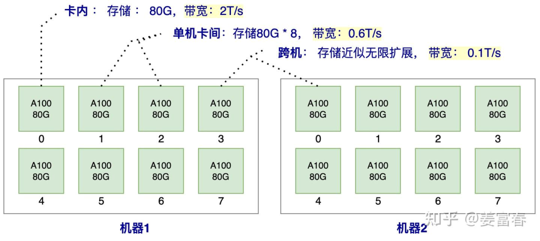
From the memory access bandwidth shown in the figure, the bandwidth within the card is three times that of single machine cards and twenty times that of cross-machine bandwidth. Therefore, we should prioritize storing data in the card, followed by within the single machine, and finally consider cross-machine storage.

Next, let’s look at what data needs to be stored in memory during the inference process.

2.2 Memory Allocation During Model Inference Stage

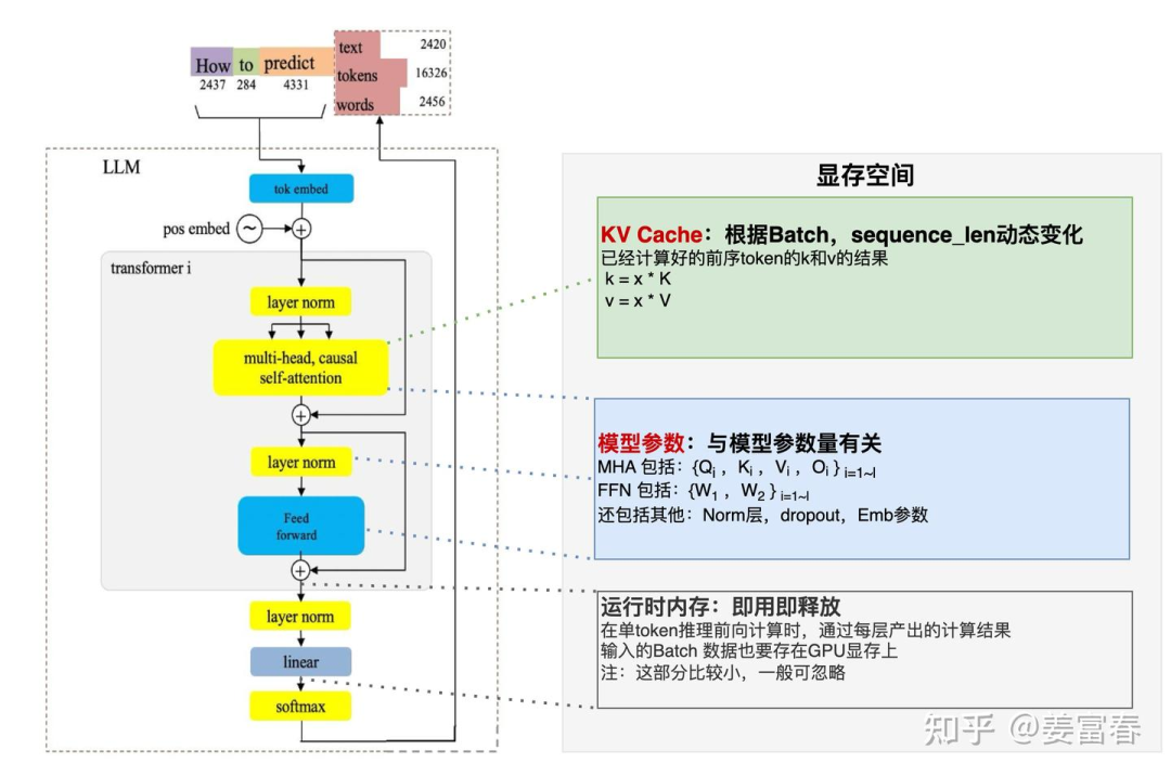
Below, I have drawn a diagram, as shown in Figure 4, where three main types of data will be stored in memory during the inference stage.

• KV Cache: As mentioned in the previous section, the results of the calculations for the preceding token sequence will gradually be stored in memory during the subsequent token inference process. The amount stored varies dynamically with Batch and Sequence_len length.
• Model Parameters: This includes parameters for the Transformer, Embedding, etc., which will be stored in memory. Once the model size is fixed, this storage space is also fixed.
• Runtime Intermediate Data: Some intermediate data produced during the inference process will be temporarily stored in memory, used and released immediately, generally occupying a relatively small space.

From the above, we can see that the main storage consumption during the inference stage is from two parts: Model Parameters and KV Cache. So how much do the model parameters occupy, and how much does the KV Cache occupy?

First, let’s take an example of the calculation process for one token to see how much KV needs to be stored for the next token. For ease of understanding, we will use the Qwen-72B model as an example, with model configuration details found at: Qwen-72B-Chat(https://huggingface.co/Qwen/Qwen-72B-Chat/blob/main/config.json).

The model has a total of 80 layers, each with 64 heads, and each head has a vector dimension of 128. Note: Here we will not consider the settings for Qwen 72B GQA (as the actual KV has undergone compression), only considering the naive MHA model structure (assuming no processing has been done), and GQA will be discussed in detail later.

As shown in Figure 5, to calculate one token, each head of each Transformer layer must store a pair of .

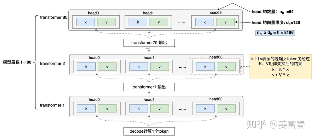
Therefore, for one token, the total amount of cached data is: where the symbols in the formula represent 1 and 1 . One token requires caching 10,240 units! Is this number a bit unexpected?

How much storage does this occupy? Assuming the model inference stage is in half-precision (bf16), each parameter occupies 2 bytes. The final storage usage for one token, as shown in formula (2): Now we know the number of cached and the storage amount required after calculating one token. For an actual inference scenario, we also need to consider the dimensions of Batch (B) and Sequence length (S) to determine the overall storage consumption of the KV Cache. These two dimensions can typically vary dynamically. Let’s look at the following two scenarios:

Scenario 1: Single Short Text Scenario

Batch and sequence settings: B = 1, S = 2048. At this time, the total cache:

Scenario 2: Concurrent Long Text Scenario

Batch and sequence settings: B = 32, S = 4096. At this time, the total cache:

In addition to the storage space consumed, we know that model parameters also occupy storage. The storage space occupied by model parameters during the inference phase is fixed and relatively simple to calculate. Assuming the parameter amount is: , with bf16 half-precision inference, the parameter amount is (Byte). Taking Qwen-72B as an example, the storage space occupied by parameters is:

Now, combining the two scenarios above, let’s look at the overall memory allocation:

• Scenario 1: Model storage, kv storage, the storage of model parameters dominates, using an 80G A100, at least 2 cards are needed for inference.
• Scenario 2: Model storage, kv storage, KV Cache storage dominates, using an 80G A100, at least 7 cards are needed for inference.

Here, I would like to elaborate a bit more. The batch size during inference depends on the offline or online business scenario, and determining the optimal batch size is a balancing process. Choosing a smaller batch size may not have high concurrency, but it may allow a single card to accommodate the complete model parameters and KV Cache, resulting in higher bandwidth on the card and potentially outstanding performance. It may be worth considering increasing the batch size to fully utilize the memory of a single card and further enhance performance. However, if the batch size increases beyond the capacity of a single card or even a single machine, the concurrency will be high, but the performance of cross-card or cross-machine memory access will decrease, leading to memory access becoming a bottleneck, resulting in inefficient use of GPU computing resources and potentially lower overall inference performance. Therefore, from the perspective of batch size settings for inference, it is essential to empirically find the optimal balance point for performance.

Current LLMs are relatively large, and memory capacity and access rates have hierarchical characteristics. Therefore, during inference, reducing cross-card and cross-machine memory read and write operations is an effective path to optimize inference performance. On one hand, the less data read and written at a time, the faster the overall speed; on the other hand, the less overall memory usage, the more data can be kept on a single card or within a single machine, allowing for higher bandwidth for data read and write operations.

The MLA we are going to study aims to compress memory usage by reducing the KV Cache, thereby optimizing inference speed. Before we delve into MLA, let’s first look at the current methods for optimizing KV Cache.

3. Methods to Reduce KV Cache

3.1 Summary of KV Cache Optimization Methods

In the industry, many methods have emerged for optimizing KV Cache. Here, I will summarize them based on my own accumulation, briefly describing the optimization ideas without going into too much detail.

There are mainly four types of methods:

1. Shared KV: Multiple heads share one set of KV, changing from one KV per head to one KV per group of heads, thus compressing KV storage. Representative methods: GQA, MQA, etc.
2. Window KV: For long sequences, control a window for computing KV, where the KV cache only saves results within the window (the window length is much smaller than the sequence length), discarding KV that exceeds the window. This method can reduce KV storage but will also lose some long text inference effectiveness. Representative methods: Longformer, etc.
3. Quantization Compression: Based on quantization methods, using lower bit rates to store KV, further compressing single KV results. Representative methods: INT8, etc.
4. Computational Optimization: By optimizing the computation process, reducing the number of memory accesses, allowing more computations to occur in on-chip SRAM to enhance inference performance. Representative methods: flashAttention, etc.

The MLA we will discuss is an optimization method under the shared KV branch. Next, let’s explore what shared KV methods exist, as these methods will also be used for comparison with MLA.

3.2 Shared KV Memory Optimization Methods

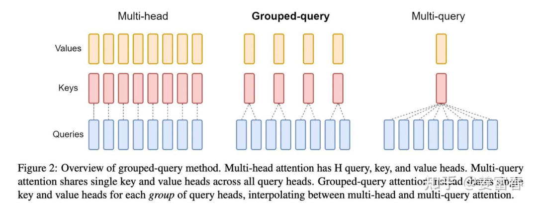
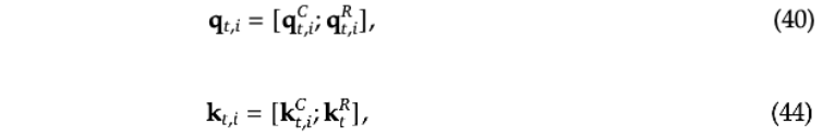
Shared KV mainly includes two methods, MQA and GQA, both proposed by Google, detailed in: MQA (2019), GQA (2023), as shown in Figure 6.

3.2.1 MQA (Multi-Query Attention)

The MQA method is relatively simple, as shown in the rightmost diagram of Figure 6, where all heads in each layer share the same to compute attention. Compared to MHA, where a single token needs to save KV numbers, it reduces to for each layer, sharing one vector and one vector.

3.2.2 GQA (Group-Query Attention)

GQA is a compromise between MQA and MHA, where not every head has one KV, nor do all heads share one KV, but rather all heads are grouped. For example, if the number of groups is , then each group shares one KV for heads. When is 1, GQA is equivalent to MQA; when is equal to the number of heads, GQA is equivalent to MHA.

To help myself better understand GQA and MQA, I will illustrate the KV calculation process for one token (as shown in Figure 5), drawing some relative details and adding annotations. As shown in Figure 7:

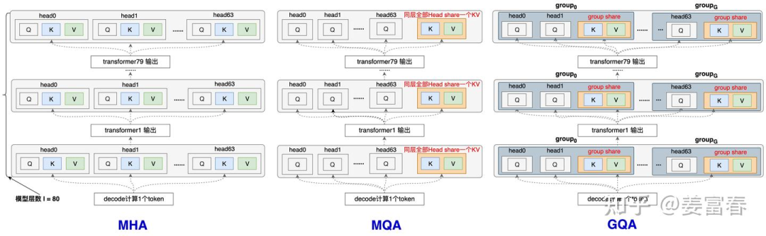
Now, let’s summarize the storage amounts of KV Cache for the various methods when calculating a single token (number of model layers: , number of heads per layer: ):

• MHA caches a total of units.
• MQA caches a total of units.
• GQA caches a total of units, where is the number of groups, and is generally a value that can be evenly divided by the number of heads.

The MLA we will discuss is also a variant of the shared KV optimization. Next, let’s look at the principles and details of MLA.

4. MLA

4.1 Overview of MLA KV Optimization

First, let’s take a quick look at the calculation method of MLA and compare the compression effects of KV with MQA and GQA.

First, let’s look at the complete formula for calculating attention in MLA, as shown in Figure 8:

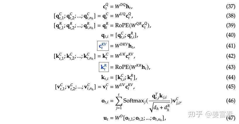
The paper mentions that each Transformer layer only caches the vectors in the blue box of the formula above: and , with dimensions:

: dimension

: dimension

Compared to MQA (where each layer has one dimension and one dimension, totaling elements), MLA effectively increases storage by 2.25 times. However, DeepSeek claims that their method is not only stronger than MQA but also superior to the original MHA without shared KV. We will discuss this further in section 4.4.

MLA is said to be fast, economical, and powerful. In the next section, we will gradually explore the specific implementation.

4.2 Understanding the Principles of MLA

Next, let’s refer to the formula in Figure 8 to examine the calculation process of MHA, first explaining the variables in the formula:

• : the dimension of low-rank compression in MLA, which is set to
• : the vector dimension of a single head
• : the number of heads per layer
• : the hidden layer dimension,
• is the low-rank transformation matrix

1. First, let’s look at the KV calculation process

• First, formula (41) performs a low-rank compression on the input , transforming the dimensional input into a dimensional . In DeepSeek-V3,
• Then, through formulas (42) and (45), the two transformation matrices (, ) expand the dimensions of KV back to , meaning each head has a separate (consistent with the number of KVs in MHA)

Note: After the above transformations, it is very similar to the logic of LoRA for low-parameter fine-tuning. By using two low-rank matrices for compression and then expansion, the number of parameters can be reduced. However, the essence of MLA is to reduce the storage of KV-cache. LoRA emphasizes the reduction of parameter quantity, and while this operation also reduces the number of parameters, according to DeepSeek-V3’s parameter configuration, the parameters of the two low-rank matrices are: , while the parameter matrix of normal MHA is: . However, MLA emphasizes the reduction of KV-cache, which means a reduction in the number of activated KV values. Currently, we cannot see how to reduce the number of activated values, as the quantity and dimensions of KV appear to be on the same level as MHA, and even more than GQA and MQA, while the computation has an additional step. This is still somewhat confusing… Let’s continue to explore…

2. Next, let’s look at the Q calculation process

Formulas (37) and (38) follow a similar logic to KV, where two matrices (, ) also perform a low-rank transformation. This step seems to be aimed at reducing the number of model parameters. In Deepseek-V3, is three times the compression dimension of KV. However, compared to , it is still significantly compressed.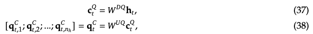

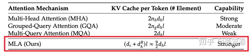
3. Adding RoPE Positional Encoding

• We note that the addition of RoPE positional encoding does not multiply the by the diagonal matrix of RoPE. Instead, two vectors with positional encoding are calculated separately, as shown in formulas (39) and (43)

Note that the calculation of the with RoPE has two details:(1) , the vector dimension is relatively small, with DeepSeek set to half the dimension of a single Attention Head: (2) This part of the calculation of is actually an MQA calculation method, where all heads in the same layer share one .

• Then, according to formulas (40) and (44), the already calculated is concatenated with the calculated to form the complete vector.

Note: The subscript here indicates the index of the Attention Head.

Thus far, we have obtained the which consists of two parts: one part is the vector obtained through low-rank compression, and the other part is the vector with positional encoding added based on MQA calculation.

Note: The principle section has already been explained very clearly by Su Shen (see: Cache and Effect Limit Pull: From MHA, MQA, GQA to MLA – Scientific Spaces), and the principle part of this article also follows Su Shen’s logic to summarize the key ideas. Thanks to Su Shen for sharing.

4.3 Comparison of MLA with MQA and GQA

Finally, let’s briefly compare the various methods, directly excerpting a diagram from the DeepSeek-V2 paper:

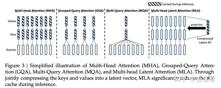
From the figure above, we can see that although the latent KV cached by MLA is relatively short (equivalent to 2.25 times the cache amount of MQA), MLA has the ability to recover the full , and its feature expression capability is significantly stronger than that of GQA and MQA. Therefore, MLA can achieve speed, economy, and power. The paper also provides the following data:

Note: Regarding the comparison of capabilities in the figure, I am somewhat skeptical about the claim that it is stronger than MHA, as I have not seen any ablation experiments for comparison, and it is also difficult to explain from a theoretical perspective.

5. Conclusion

This article attempts to introduce more foundational knowledge and auxiliary information to gain a deeper understanding of MLA. The content is relatively long and may seem somewhat verbose. This is a recursive summary of some extended information during my understanding of MLA, ultimately organizing a systematic context to share for everyone’s reference.

6. References

[1] deepseek-v1: https://arxiv.org/pdf/2401.02954[2] deepseek-v2: https://arxiv.org/pdf/2405.04434[3] deepseek-v3: https://arxiv.org/pdf/2412.19437[4] Cache and Effect Limit Pull: From MHA, MQA, GQA to MLA – Scientific Spaces (https://spaces.ac.cn/archives/10091)[5] https://zhuanlan.zhihu.com/p/659770503[6] GQA: https://arxiv.org/pdf/2305.13245[7] MQA: https://arxiv.org/pdf/1911.02150