Reinforcement Learning for Autonomous 3D Control of Magnetic Microrobots

Keywords: Microrobots, Biomedical Engineering, Reinforcement Learning

Paper Title: Autonomous 3D positional control of a magnetic microrobot using reinforcement learning

Journal: Nature Machine Intelligence

Paper Link: https://www.nature.com/articles/s42256-023-00779-2

The small size of microrobots allows them to access all parts of the body, facilitating targeted treatment and diagnosis. Recent studies have revealed the enormous potential of microrobots in biomedical engineering and medicine. However, the small size of microrobots poses limitations for built-in electronic devices, making wireless operation feasible only through optical, chemical, or magnetic means. Given their high permeability, biocompatibility, and good degrees of freedom control, magnetic actuation is the preferred method. This study employs reinforcement learning to achieve autonomous 3D positional control of magnetic microrobots.

Magnetic microrobots have shown potential in biomedical engineering, facilitating precise drug delivery, non-invasive diagnostics, and cell-based therapies. Currently, the technology controlling the motion of such microrobots relies on the assumption of a uniform magnetic field and is significantly affected by the characteristics of the microrobots and the surrounding environment. These strategies lack universality and adaptability when the environment or microrobots change, and moderate delays occur due to the independent control of the electromagnetic drive system and the microrobot’s position.

To address these issues, this study proposes a method to control the position of magnetic microrobots through a gradient field generated by electromagnetic coils based on machine learning. The study uses reinforcement learning and progressive training methods to control the 3D position of microrobots within a defined workspace by directly managing coil currents. A simulation environment was developed for initial exploration to reduce overall training time. After simulation training, the learning process was transferred to a physical electromagnetic drive system that reflects the complexities of the real world. The proposed method is more accurate and efficient compared to traditional proportional-integral-derivative control (PID control). Additionally, this method integrates path planning algorithms to achieve fully autonomous control. Furthermore, this method serves as an alternative to complex mathematical models that are highly sensitive to the nonlinearity of microrobot design, environment, and magnetic systems.

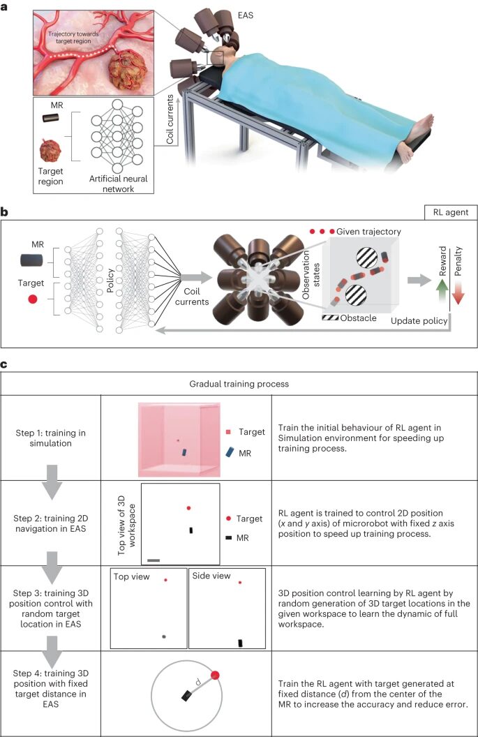
Figure 1 a, Navigation of magnetic microrobots based on reinforcement learning. This study developed an autonomous method to navigate microrobots in complex environments using reinforcement learning to control the external actuation system (EAS). b, The RL agent precisely controls the position of the MR by changing the EAS coil current. The MR reaches the target position PT in the least number of steps according to the policy π (neural network, part of the RL agent), while maintaining within the defined workspace region of interest (ROI). c, A four-step training process was adopted in this study to reduce the training time of the agent and improve accuracy. This aids in initial exploration and gradually increases complexity, ensuring accurate navigation.

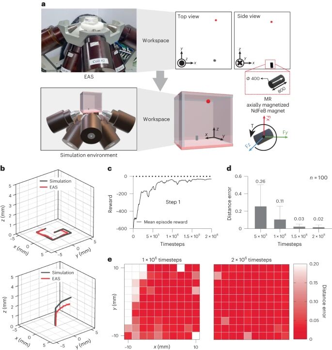
Figure 2 Evaluation and training results in a simulation environment. a, A simulation environment developed in Unity 3D for an EAS with eight coils and a magnetic microrobot (a permanent magnet with a south-to-north magnetization direction, as indicated by the white arrow) immersed in 350cSt silicone oil, with NdFeB representing neodymium-iron-boron material. b, Environment evaluation. c, Training results of the reinforcement learning agent model in the first step of the training process, represented by the average reward value changing over time steps. d, Distance error (distance from the microrobot to the target point) changes as the reinforcement learning agent navigates through different training steps. e, A heatmap of distance error across the entire workspace.

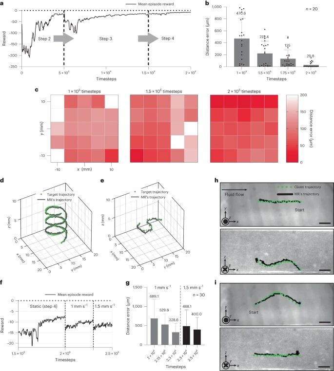
Figure 3 Retraining the reinforcement learning agent model using EAS (real environment). a, The RL agent was retrained with EAS for 2×106 time steps, with training conditions changed after each saturation point (steps 2-4). b, Distance error (distance from the microrobot to the target point) changes as the reinforcement learning agent navigates the MR through various training intervals. c, A heatmap of distance error across the entire workspace. d, The spiral trajectory given to the reinforcement learning agent for navigating the microrobot. This task involves changes across three axes, validating the agent’s performance. e, The MR navigates along an S-shaped trajectory in the xy-plane; the z-axis is fixed. This method validates the hovering capability of the reinforcement learning agent. f, The RL agent was retrained under fluid flow conditions, involving 300,000 and 200,000 time steps at fluid speeds of 1 mm/s and 1.5 mm/s respectively. g, Distance error during retraining in a dynamic fluid environment at two different speeds. h, Navigation against fluid flow (1 mm/s). i, Navigation with fluid flow (1 mm/s).

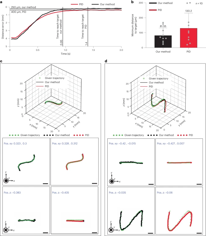
Figure 4 Comparison of the method with closed-loop control using PID controller. a, Using both methods, a target point 4mm away from the current MR position was created to evaluate the time required to reach the target point. b, The accuracy was compared by navigating the MR to random target points and recording the minimum distance to the target point. c, Trajectories used to compare the hovering performance (fixed z-axis). d, Trajectories used to assess performance under gravity (fixed y-axis).

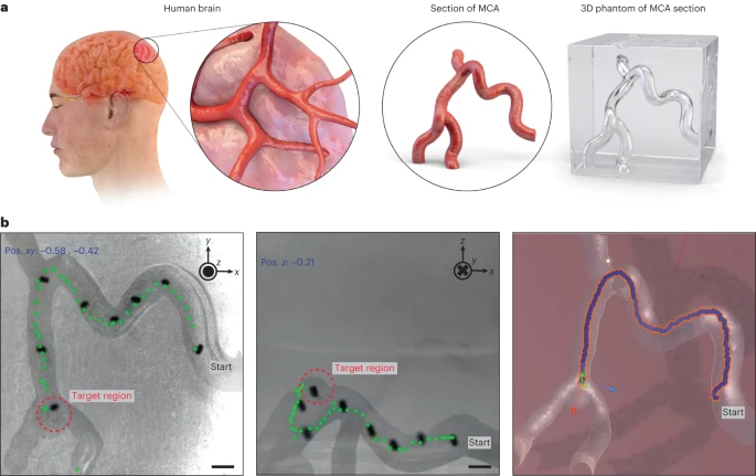
Figure 5 Navigating MR in a cerebral vascular simulation model. a, A scaled replica of the MCA cross-section as a cerebral vascular simulation model, used to evaluate the performance of the RL agent as a potential medical application. b, The RL agent navigates from a specified starting point to the target point, which is an aneurysm within the simulation model.

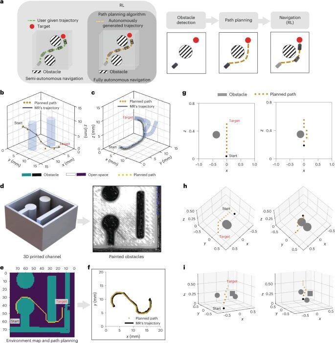
Figure 6 Fully autonomous control of MR in different environments. a, The RL agent generates optimal currents for 3D closed-loop position control (assuming nonlinear systems and nonlinear environments) as the “brain” (the navigation trajectory is human-selected). The RL agent merges with path planning algorithms to generate trajectories towards the target; this constitutes fully autonomous control. b, c, Two different MR navigation scenarios using trajectories generated by A*: the first includes virtual obstacles (two cylinders) (b), and the second includes a 3D virtual channel (c). d, Environmental mapping using image processing to detect obstacles and open spaces. A cube channel with obstacles was used to test path planning and navigation. e, Results of path planning. f, Navigating through a channel with physical obstacles. g, h, i, MR navigation encountering a single dynamic obstacle (g), two dynamic obstacles (h), and two dynamic obstacles plus one static obstacle (i).

Using deep reinforcement learning combined with neural network strategies can model complex problems. This study employed a model-free reinforcement learning approach to control the navigation of magnetic MR. Reinforcement learning can explore problems beyond expert understanding and effectively solve them. The researchers proposed a stepwise training process to address the main issues of long training times requiring manual intervention and irreversible system states encountered when training with reinforcement learning in physical environments, reducing overall training time and improving accuracy. Consequently, the reinforcement learning agent learned to control the position of the MR, navigating it to defined targets within the workspace. Meanwhile, training was conducted using the flow generated by a peristaltic pump within fluid channels, and the method’s potential in dynamic fluid environments was also tested, indicating that the trained strategy could serve as a universal strategy for navigating gradient-type MR, allowing for retraining the reinforcement learning agent to adapt to various MRs. Compared to PID controllers, this method achieved significantly higher accuracy and shorter target reach times. Additionally, this method enabled fully autonomous navigation around static and dynamic obstacles.

In the future, the researchers believe this method has the potential to help control the position, direction, and speed of MRs in 3D dynamic environments within rotating and oscillating magnetic fields. This technology could also expand the operational workspace of existing EAS by focusing on MRs trained in non-uniform magnetic fields away from the center. This method can be combined with various imaging and magnetic drive systems, as well as algorithms that facilitate 3D path planning and navigation. This combination would extend the method to practical medical imaging applications and experiments.

Compiled by | Yu Mengjun

Reading Club on Large Language Models and Multi-Agent Systems

For more details, see:

Reading Club on Large Language Models and Multi-Agent Systems: Large Models Empowering Robots to Emerge Collective Intelligence

Recommended Reading

1. Reconfigurable Microscopic Swarm Robots Illuminate the Future of Medicine and Environmental Remediation

2. Biologically Mixed Robots Made from Cells – The Next Frontier in Robotics

3.Long Review: The Past, Present, and Future of Swarm Robotics

4. Zhangjiang: The Foundation of Third-Generation AI Technology – From Differentiable Programming to Causal Inference | New Course by Collective Intelligence Academy

5. Join Collective Intelligence Academy VIP to Access All Content Resources on the Platform

6. Join Collective Intelligence, Let’s Get Complex!

Click “Read Original” to Register for the Reading Club