Basic Concepts
To understand I/O, we first need to grasp a few concepts: file system, disk, and file..
Disk
The disk provides the most basic persistent storage capability for the system.
Classification of Disks
Based on the storage medium, disks can be classified into two categories: mechanical disks and solid-state disks.
Mechanical Disk: Composed of platters and read/write heads. Data is stored in the circular tracks of the platters. When reading or writing data, the read/write head must first move to the corresponding track before accessing the data.
Solid-State Disk: Composed of solid-state electronic components, solid-state drives do not require track addressing.
From the above, we can conclude:
1. Mechanical disks consume seek time and reduce efficiency when accessing non-contiguous data, while solid-state disks do not.
2. Whether mechanical or solid-state, sequential I/O is faster than random I/O.
-
General block layer strategies can merge contiguous I/O requests to improve efficiency.
-
Utilize the caching mechanism of the file system.
Performance Metrics
To measure disk performance, five common metrics must be mentioned.
-
Utilization: Refers to the percentage of time the disk is processing I/O. Note that even at 100% utilization, the disk may still accept new I/O requests.
-
Saturation: Refers to the level of busyness of the disk in processing I/O. Note that when saturation reaches 100%, the disk cannot accept new I/O requests.
-
IOPS (Input/Output Per Second): The number of I/O requests per second.
-
Throughput: Refers to the size of I/O requests per second.
-
Response Time: Refers to the time interval from when an I/O request is issued to when a response is received.
Ways to View Performance Metrics
yihua@ubuntu:~$ iostat -d -x 1Linux 4.15.0-213-generic (ubuntu) 10/30/2023 _x86_64_ (4 CPU)Device r/s w/s rkB/s wkB/s rrqm/s wrqm/s %rrqm %wrqm r_await w_await aqu-sz rareq-sz wareq-sz svctm %utilloop0 0.00 0.00 0.01 0.00 0.00 0.00 0.00 0.00 0.50 0.00 0.00 1.85 0.00 0.02 0.00loop1 0.00 0.00 0.00 0.00 0.00 0.00 0.00 0.00 1.06 0.00 0.00 4.08 0.00 0.00 0.00loop2 0.00 0.00 0.01 0.00 0.00 0.00 0.00 0.00 0.33 0.00 0.00 2.11 0.00 0.01 0.00loop3 0.00 0.00 0.00 0.00 0.00 0.00 0.00 0.00 10.22 0.00 0.00 2.50 0.00 0.00 0.00loop4 0.00 0.00 0.00 0.00 0.00 0.00 0.00 0.00 1.06 0.00 0.00 4.09 0.00 0.07 0.00loop5 0.00 0.00 0.00 0.00 0.00 0.00 0.00 0.00 2.57 0.00 0.00 2.57 0.00 0.00 0.00loop6 0.05 0.00 0.05 0.00 0.00 0.00 0.00 0.00 2.69 0.00 0.00 1.06 0.00 0.05 0.00loop7 0.00 0.00 0.00 0.00 0.00 0.00 0.00 0.00 1.20 0.00 0.00 2.25 0.00 0.03 0.00sda 0.38 0.61 11.59 44.20 0.07 0.63 15.21 50.81 0.81 4.16 0.00 30.82 72.85 0.25 0.02scd0 0.00 0.00 0.00 0.00 0.00 0.00 0.00 0.00 0.08 0.00 0.00 3.75 0.00 0.08 0.00scd1 0.00 0.00 0.00 0.00 0.00 0.00 0.00 0.00 0.13 0.00 0.00 17.48 0.00 0.13 0.00loop8 0.00 0.00 0.00 0.00 0.00 0.00 0.00 0.00 10.22 0.00 0.00 2.50 0.00 0.00 0.00loop9 0.00 0.00 0.00 0.00 0.00 0.00 0.00 0.00 0.75 0.00 0.00 3.19 0.00 0.02 0.00loop10 0.00 0.00 0.00 0.00 0.00 0.00 0.00 0.00 11.20 0.00 0.00 2.35 0.00 0.00 0.00loop11 0.00 0.00 0.00 0.00 0.00 0.00 0.00 0.00 0.88 0.00 0.00 3.41 0.00 0.06 0.00loop12 0.00 0.00 0.00 0.00 0.00 0.00 0.00 0.00 4.63 0.00 0.00 2.47 0.00 0.00 0.00loop13 0.00 0.00 0.00 0.00 0.00 0.00 0.00 0.00 1.23 0.00 0.00 4.51 0.00 0.08 0.00loop14 0.00 0.00 0.00 0.00 0.00 0.00 0.00 0.00 2.37 0.00 0.00 3.23 0.00 0.44 0.00loop15 0.00 0.00 0.00 0.00 0.00 0.00 0.00 0.00 0.68 0.00 0.00 3.39 0.00 0.06 0.00loop16 0.00 0.00 0.00 0.00 0.00 0.00 0.00 0.00 1.58 0.00 0.00 4.61 0.00 0.19 0.00loop17 0.00 0.00 0.00 0.00 0.00 0.00 0.00 0.00 0.80 0.00 0.00 2.23 0.00 0.08 0.00loop18 0.00 0.00 0.00 0.00 0.00 0.00 0.00 0.00 27.00 0.00 0.00 1.00 0.00 0.00 0.00loop19 0.00 0.00 0.00 0.00 0.00 0.00 0.00 0.00 1.96 0.00 0.00 2.19 0.00 0.07 0.00loop20 0.00 0.00 0.00 0.00 0.00 0.00 0.00 0.00 2.82 0.00 0.00 2.41 0.00 0.00 0.00loop21 0.00 0.00 0.00 0.00 0.00 0.00 0.00 0.00 1.43 0.00 0.00 4.57 0.00 0.07 0.00loop22 0.00 0.00 0.00 0.00 0.00 0.00 0.00 0.00 2.18 0.00 0.00 2.97 0.00 0.37 0.00loop23 0.00 0.00 0.00 0.00 0.00 0.00 0.00 0.00 0.56 0.00 0.00 2.17 0.00 0.03 0.00loop24 0.00 0.00 0.00 0.00 0.00 0.00 0.00 0.00 5.91 0.00 0.00 2.57 0.00 0.00 0.00loop25 0.00 0.00 0.00 0.00 0.00 0.00 0.00 0.00 0.37 0.00 0.00 2.91 0.00 0.02 0.00loop26 0.00 0.00 0.00 0.00 0.00 0.00 0.00 0.00 5.80 0.00 0.00 2.35 0.00 0.00 0.00loop27 0.00 0.00 0.00 0.00 0.00 0.00 0.00 0.00 0.00 0.00 0.00 1.60 0.00 0.00 0.00File System
The file system provides a tree structure for managing files based on the disk. It is a mechanism for organizing and managing files on storage devices. Different organizational methods lead to different file systems.
File
For easier management, the file system allocates two data structures for files: inode and directory structure.
-
Inode: Short for index node, it records the metadata of the file, such as inode number, file size, access permissions, modification date, data location, etc. Each inode corresponds to a file, and like file content, it is persistently stored on the disk. Therefore, inodes occupy disk space.
-
Directory Entry: Short for dentry, it records the file name, inode pointer, and the relationships between other directory entries. Multiple related directory entries form the directory structure of the file system.
From the above, we can conclude:
-
Inodes and directory entries also occupy disk space. Moreover, there is a limit to the number of inodes and directory entries in the file system. Therefore, if there are a large number of small files in a Linux system, there may still be free disk space, but it may not be possible to create new files.
-
The relationship between directory entries and inodes is many-to-one. That is, a file can have multiple aliases, such as hard links in a Linux system.
File I/O
Based on the method of accessing files, I/O can be classified into several types, with the following four being common.
-
Buffered I/O/Unbuffered I/O: Here, buffering refers to application-level caching, as some standard libraries have caching mechanisms to reduce the number of I/O operations. For example, printf only outputs when it encounters a newline character because the content before the newline is cached by the standard library; at this point, the content is still at the application level and has not reached the kernel.
-
Direct I/O/Non-Direct I/O: The file system caches data to speed up read and write operations. Based on specific mechanisms (such as cache full, system calls, cache expiration, disk write requests, or cache flushing), the cache is written to the disk, which is what I often refer to as the disk write mechanism. Direct I/O specifies the O_DIRECT flag during the system call, indicating that the file system’s caching mechanism should not be used.
-
Blocking I/O/Non-Blocking I/O: This refers to whether the application thread is blocked after executing a system call if no result is obtained. For example, when accessing a pipe or network socket, setting the O_NONBLOCK flag indicates that non-blocking access is used.
-
Synchronous I/O/Asynchronous I/O: This refers to whether the application needs to wait for the I/O operation to complete or respond after executing an I/O operation. For example, when operating on a file, if you set O_DSYNC, you must wait for the file data to be written to the disk before returning.
In the above descriptions, buffered I/O and direct I/O are relatively easy to understand and distinguish. However, how do we differentiate between blocking I/O and synchronous I/O?
My understanding is:
-
Blocking I/O is an active behavior of the application. It actively releases held resources, such as CPU or file descriptors.
-
Synchronous I/O is a passive behavior of the application. It waits for events to be satisfied and does not release resources during the waiting process.
Performance Analysis
Regarding the file system, we generally care about two performance parameters: capacity and cache.
-
Capacity
We can check the current remaining size of the file system using the df command.
yihua@ubuntu:~$ df -hFilesystem Size Used Avail Use% Mounted onudev 1.9G 0 1.9G 0% /devtmpfs 392M 3.6M 389M 1% /run/dev/sda1 49G 42G 4.5G 91% /tmpfs 2.0G 0 2.0G 0% /dev/shmtmpfs 5.0M 4.0K 5.0M 1% /run/locktmpfs 2.0G 0 2.0G 0% /sys/fs/cgroup/dev/loop1 219M 219M 0 100% /snap/gnome-3-34-1804/93/dev/loop3 512K 512K 0 100% /snap/gnome-characters/789/dev/loop2 82M 82M 0 100% /snap/gtk-common-themes/1534/dev/loop16 106M 106M 0 100% /snap/core/15925/dev/loop5 1.5M 1.5M 0 100% /snap/gnome-system-monitor/184/dev/loop10 896K 896K 0 100% /snap/gnome-logs/121/dev/loop11 141M 141M 0 100% /snap/gnome-3-26-1604/111/dev/loop12 2.3M 2.3M 0 100% /snap/gnome-calculator/953/dev/loop8 512K 512K 0 100% /snap/gnome-characters/795/dev/loop13 74M 74M 0 100% /snap/core22/858/dev/loop18 128K 128K 0 100% /snap/bare/5/dev/loop14 350M 350M 0 100% /snap/gnome-3-38-2004/143/dev/loop19 64M 64M 0 100% /snap/core20/2015/dev/loop23 64M 64M 0 100% /snap/core20/1974/dev/loop20 2.2M 2.2M 0 100% /snap/gnome-calculator/950/dev/loop24 1.7M 1.7M 0 100% /snap/gnome-system-monitor/186/dev/loop21 74M 74M 0 100% /snap/core22/864/dev/loop7 56M 56M 0 100% /snap/core18/2790/dev/loop26 896K 896K 0 100% /snap/gnome-logs/119/dev/loop25 486M 486M 0 100% /snap/gnome-42-2204/126/dev/loop15 141M 141M 0 100% /snap/gnome-3-26-1604/104/dev/loop0 92M 92M 0 100% /snap/gtk-common-themes/1535/dev/loop4 219M 219M 0 100% /snap/gnome-3-34-1804/90/dev/loop6 106M 106M 0 100% /snap/core/16202/dev/loop9 350M 350M 0 100% /snap/gnome-3-38-2004/140/dev/loop22 497M 497M 0 100% /snap/gnome-42-2204/141tmpfs 392M 28K 392M 1% /run/user/121tmpfs 392M 36K 392M 1% /run/user/1000/dev/sr1 1.9G 1.9G 0 100% /media/yihua/Ubuntu 18.04.1 LTS amd64/dev/sr0 46M 46M 0 100% /media/yihua/CDROM/dev/loop27 56M 56M 0 100% /snap/core18/2796Note: The size displayed by the file system does not equal the size of the disk.
-
Cache
We can check the current cache size using the free command.
yihua@ubuntu:~$ free -h total used free shared buff/cache availableMem: 3.8G 1.3G 1.5G 31M 1.1G 2.3GSwap: 2.0G 87M 1.9GHowever, our file system mainly has three types of caches: page cache, inode cache, and directory entry cache. These parameters cannot be directly obtained from the free command. Therefore, details need to be obtained from /proc/meminfo.
yihua@ubuntu:~$ cat //proc/meminfoMemTotal: 4013248 kBMemFree: 1576180 kBMemAvailable: 2400348 kBBuffers: 97364 kBCached: 906452 kBSwapCached: 3840 kBActive: 795076 kBInactive: 1181056 kBActive(anon): 376460 kBInactive(anon): 628448 kBAmong them, Cached is the sum of the three caches, and you can view more detailed content using slabtop
Active / Total Objects (% used) : 989070 / 1045443 (94.6%) Active / Total Slabs (% used) : 20382 / 20382 (100.0%) Active / Total Caches (% used) : 84 / 114 (73.7%) Active / Total Size (% used) : 242473.95K / 262634.13K (92.3%) Minimum / Average / Maximum Object : 0.01K / 0.25K / 8.00K OBJS ACTIVE USE OBJ SIZE SLABS OBJ/SLAB CACHE SIZE NAME 51145 47067 0% 0.60K 965 53 30880K inode_cache 56192 55803 0% 0.50K 878 64 28096K kmalloc-512145020 144307 0% 0.13K 2417 60 19336K kernfs_node_cache 17168 13103 0% 1.07K 592 29 18944K ext4_inode_cache 93870 76404 0% 0.19K 2235 42 17880K dentry 29792 21524 0% 0.57K 532 56 17024K radix_tree_nodeFrom the above, the directory entry and inode cache occupy about 32M.
I/O Stack
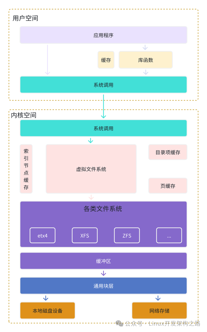
Virtual File System
As shown in the figure above, to support different file systems, the Linux kernel introduces an abstraction layer between user space and the file system, known as the Virtual File System (VFS).
VFS defines the data structures and standard interfaces supported by all file systems. This way, user processes only need to interact with the unified interface provided by VFS, without needing to care about the implementation details of various underlying file systems.
Below VFS, Linux supports a variety of file systems. Based on storage location, these file systems can be divided into three categories.
-
The first category is disk-based file systems, which store data directly on the locally mounted disks of the computer. Common examples include Ext4, XFS, OverlayFS, etc.
-
The second category is memory-based file systems, commonly referred to as virtual file systems. These file systems do not require any disk allocation for storage but will occupy memory. The /proc file system we often use is actually one of the most common virtual file systems. Additionally, the /sys file system also belongs to this category, mainly exporting hierarchical kernel objects to user space.
-
The third category is network file systems, which are used to access data from other computers, such as NFS, SMB, iSCSI, etc.
These file systems must first be mounted to a subdirectory in the VFS directory tree (called a mount point) before their files can be accessed.
General Block Layer
Similar to the Virtual File System (VFS), to reduce the impact of differences between different block devices, Linux manages various block devices through a unified general block layer.
The general block layer is an abstraction layer for block devices that sits between the file system and disk drivers. It mainly has two functions:
-
Upward, it provides a standard interface for file systems and applications to access block devices; downward, it abstracts various heterogeneous disk devices into a unified block device and provides a unified framework to manage the drivers of these devices.
-
Block devices will also queue the I/O requests sent to them and improve disk efficiency through reordering, request merging, etc.
Among them, there are four types of sorting algorithms:
-
NONE: No processing is done.
-
NOOP: Essentially a first-in-first-out queue, with basic request merging on top of that.
-
CFQ: Completely Fair Queuing, which is the default I/O scheduling policy for many distributions. It maintains an I/O queue for each process and evenly distributes each process’s I/O requests according to time slices.
-
Deadline: It creates different I/O queues for read and write requests, which can improve the throughput of mechanical disks and ensure that requests with deadlines are prioritized. This is often used in scenarios with heavy I/O pressure, such as databases.
If you are learning Linux C++ development technology, here is a share of learning materials for Linux C++. The materials include C++ Linux development video tutorials, complete C++ learning paths, C++ interview questions from major companies, etc. Scan the QR code below to receive them for free.Tool Introduction
During the I/O performance analysis process, we need to use some tools to assist us in analyzing, locating, and solving problems.
top
The top command is a commonly used tool when analyzing performance issues. Execute top -d 1, where the -d parameter indicates the update frequency. The default is 3 seconds.
yihua@ubuntu:~$ top -d 1top - 23:36:05 up 22:14, 4 users, load average: 0.48, 0.10, 0.03Tasks: 330 total, 1 running, 253 sleeping, 0 stopped, 0 zombie%Cpu(s): 9.9 us, 66.5 sy, 0.0 ni, 23.6 id, 0.0 wa, 0.0 hi, 0.0 si, 0.0 stKiB Mem : 4013240 total, 1004708 free, 1293040 used, 1715492 buff/cacheKiB Swap: 2097148 total, 2097148 free, 0 used. 2398648 avail Mem Unknown command - try 'h' for help PID USER PR NI VIRT RES SHR S %CPU %MEM TIME+ COMMAND 10612 yihua 20 0 120024 7940 6636 S 305.0 0.2 0:21.79 sysbench 10623 yihua 20 0 44380 4132 3328 R 1.0 0.1 0:00.03 top 1 root 20 0 225544 9332 6636 S 0.0 0.2 0:03.29 systemd 2 root 20 0 0 0 0 S 0.0 0.0 0:00.04 kthreadd 4 root 0 -20 0 0 0 I 0.0 0.0 0:00.00 kworker/0:0H 6 root 0 -20 0 0 0 I 0.0 0.0 0:00.00 mm_percpu_wq 7 root 20 0 0 0 0 S 0.0 0.0 0:00.09 ksoftirqd/0 8 root 20 0 0 0 0 I 0.0 0.0 0:00.61 rcu_sched 9 root 20 0 0 0 0 I 0.0 0.0 0:00.00 rcu_bh 10 root rt 0 0 0 0 S 0.0 0.0 0:00.00 migration/0 11 root rt 0 0 0 0 S 0.0 0.0 0:00.09 watchdog/0The third line:%Cpu(s): 9.9 us, 66.5 sy, 0.0 ni, 23.6 id, 0.0 wa, 0.0 hi, 0.0 si, 0.0 st
Indicates the current CPU resource consumption status. The parameters can be referenced as follows:
user (usually abbreviated as us) represents user mode CPU time. Note that it does not include nice time but includes guest time.That is, executing user mode code..
nice (usually abbreviated as ni) represents low-priority user mode CPU time, which is the CPU time when the process’s nice value is adjusted to between 1-19. Note that the nice value can range from -20 to 19, with higher values indicating lower priority.Executing user mode code..
system (usually abbreviated as sys) represents kernel mode CPU time.Executing kernel mode code..
idle (usually abbreviated as id) represents idle time. Note that it does not include time spent waiting for I/O (iowait).
iowait (usually abbreviated as wa) represents CPU time spent waiting for I/O.Duration of processes in an uninterruptible state..
irq (usually abbreviated as hi) represents CPU time spent handling hardware interrupts.Executing hardware interrupt code..
softirq (usually abbreviated as si) represents CPU time spent handling software interrupts.Executing software interrupt code..
steal (usually abbreviated as st) represents CPU time occupied by other virtual machines when the system is running in a virtual machine.
-
Using the top command, we can confirm whether there are I/O performance issues in the current system.
iostat
The iostat command can view the status of all file systems in the system.
# -d indicates to display I/O performance metrics, -x indicates to display extended statistics (i.e., all I/O metrics) $ iostat -x -d 1 Device r/s w/s rkB/s wkB/s rrqm/s wrqm/s %rrqm %wrqm r_await w_await aqu-sz rareq-sz wareq-sz svctm %util loop0 0.00 0.00 0.00 0.00 0.00 0.00 0.00 0.00 0.00 0.00 0.00 0.00 0.00 0.00 0.00 sdb 0.00 0.00 0.00 0.00 0.00 0.00 0.00 0.00 0.00 0.00 0.00 0.00 0.00 0.00 0.00 sda 0.00 64.00 0.00 32768.00 0.00 0.00 0.00 0.00 0.00 7270.44 1102.18 0.00 512.00 15.50 99.20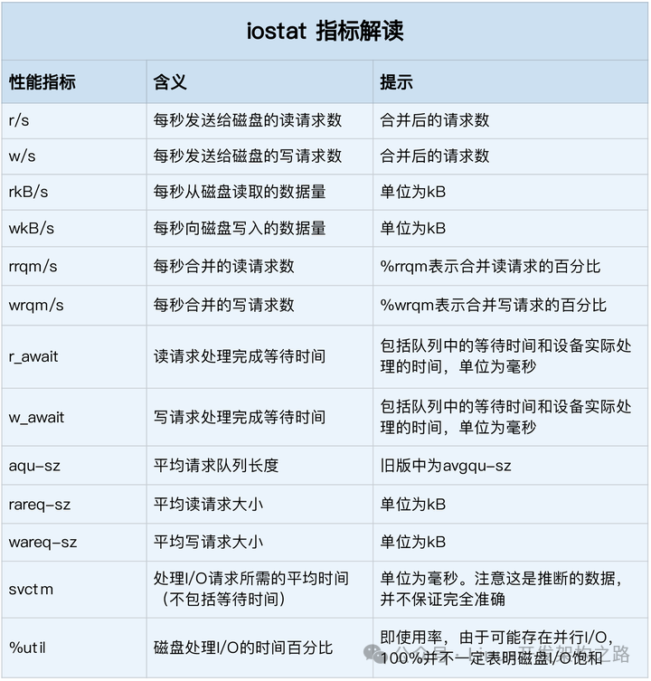
In the disk performance metrics section, the metrics for measuring disk performance include utilization, saturation, IOPS, throughput, and response time. The corresponding relationships are as follows:
-
Utilization (%util)
-
Saturation: Saturation usually does not have other simple observation methods.
-
IOPS (r/s + w/s)
-
Throughput (rkB/s + wkB/s)
-
Response Time (r_await + w_await)
From the above, it can be seen that the current sda disk is experiencing a performance bottleneck, mainly reflected in high utilization and a write request response time of 7 seconds.
-
From the above, it can be seen that through iostat, we can quickly locate which disk is experiencing an I/O performance bottleneck and confirm which type of I/O operation is causing the bottleneck.
pidstat
The pidstat command can help us observe the I/O status of processes.
$ pidstat -d 1 13:39:51 UID PID kB_rd/s kB_wr/s kB_ccwr/s iodelay Command 13:39:52 102 916 0.00 4.00 0.00 0 rsyslogdFrom the output of pidstat, you can see that it can view the I/O situation of each process in real-time, including the following content.
-
User ID (UID) and Process ID (PID). The size of data read per second (kB_rd/s), in KB.
-
The size of data written per second (kB_wr/s), in KB.
-
The size of canceled write requests per second (kB_ccwr/s), in KB.
-
Block I/O delay (iodelay), including the time spent waiting for synchronous block I/O and the time spent waiting for block I/O to finish, measured in clock cycles.
From the above, we can locate which process is causing high I/O load through pidstat.
strace
The strace command can view the system calls of a process. According to the I/O stack, applications must enter kernel mode through system calls to perform I/O requests.
$ strace -f -p 18940 strace: Process 18940 attached ...mmap(NULL, 314576896, PROT_READ|PROT_WRITE, MAP_PRIVATE|MAP_ANONYMOUS, -1, 0) = 0x7f0f7aee9000 mmap(NULL, 314576896, PROT_READ|PROT_WRITE, MAP_PRIVATE|MAP_ANONYMOUS, -1, 0) = 0x7f0f682e8000 write(3, "2018-12-05 15:23:01,709 - __main"..., 314572844 ) = 314572844 munmap(0x7f0f682e8000, 314576896) = 0 write(3, "\n", 1) = 1 munmap(0x7f0f7aee9000, 314576896) = 0 close(3) = 0 stat("/tmp/logtest.txt.1", {st_mode=S_IFREG|0644, st_size=943718535, ...}) = 0From the output of strace, it can be determined that the current I/O operation is mainly a write operation, and the corresponding file socket is 3.
-
From the above, it can be seen that the strace command can observe the system calls of a process and their associated file sockets.
lsof
The lsof command is specifically used to view the list of open files for a process. However, here, “files” include not only ordinary files but also directories, block devices, dynamic libraries, network sockets, etc.
$ lsof -p 18940 COMMAND PID USER FD TYPE DEVICE SIZE/OFF NODE NAME python 18940 root cwd DIR 0,50 4096 1549389 / python 18940 root rtd DIR 0,50 4096 1549389 / … python 18940 root 2u CHR 136,0 0t0 3 /dev/pts/0 python 18940 root 3w REG 8,1 117944320 303 /tmp/logtest.txt From the above, file socket 3 corresponds to /tmp/logtest.txt, thus allowing us to identify the corresponding code block.
I/O Performance Optimization Strategies
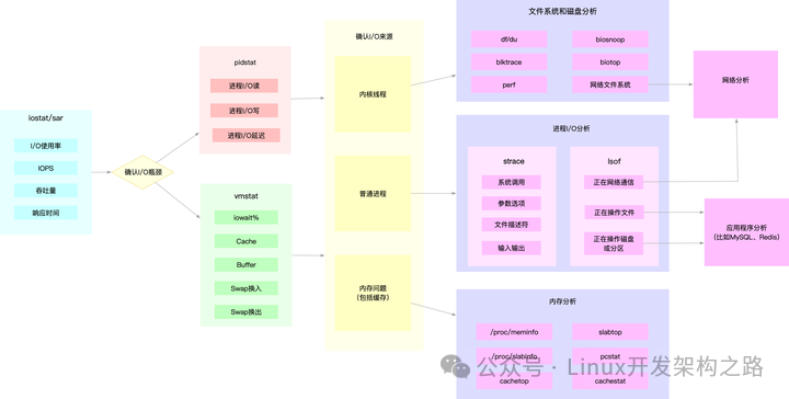
By using iostat to check the I/O status of the system disk. If an I/O performance bottleneck occurs, the response time will typically be high.
1. If there is high throughput, IOPS, and utilization, it indicates that processes are performing I/O operations.
Using pidstat can quickly locate which process is performing I/O operations.
If it is a kernel process, it is generally caused by external environments, such as frequent external device interactions or abnormal network conditions.
If it is an application process, use strace + lsof to confirm what the current process is doing.
-
If it is performing network communication, analyze the network environment.
-
If it is performing file operations or disk operations, analyze the application.
2. If only the response time is high but throughput, IOPS, and utilization are normal, it may be due to memory issues, as insufficient memory can also lead to I/O response delays.
-
Use vmstat + /proc/meminfo to analyze which cache is abnormal and take action accordingly.
Common Optimization Measures
Application Layer Optimization
-
Use append writes instead of random writes to reduce addressing overhead.
-
Utilize buffered I/O to make full use of system cache and reduce actual I/O operations. For example, do not use the O_DIRECT parameter when opening files.
-
Create application-level caches, similar to external caching systems like Redis. For example, the C standard library provides functions like fopen, fread, etc., which utilize standard library caching to reduce disk operations.
-
For frequent read/write operations, use mmap instead of read/write to reduce memory copy times.
-
Try to merge write requests instead of synchronously writing each request to the disk; you can use fsync() instead of O_SYNC.
-
Set I/O scheduling algorithms based on business scenario requirements. If using the CFQ algorithm, you can set the priority of the application.
File System Optimization
-
Select the most suitable file system based on the load. For example, compared to ext4, xfs supports larger disk partitions and more files, such as xfs supporting disks larger than 16TB. However, the downside of the xfs file system is that it cannot be shrunk, while ext4 can.
-
Optimize the caching of the file system.
-
When persistence is not required, you can also use the memory file system tmpfs.
Disk Optimization
-
Replace with higher-performance disks, such as replacing HDDs with SSDs.
-
Isolate application data at the disk level. For example, log and database programs require frequent read/write operations. We can configure separate disks for them.
-
In scenarios with more sequential reads, we can increase the pre-read data of the disk. Adjust the kernel option /sys/block/sdb/queue/read_ahead_kb, the default size is 128 KB, measured in KB.
-
Optimize kernel block device I/O options. For example, adjust the length of the disk queue. /sys/block/sdb/queue/nr_requests, appropriately increasing the queue length can improve disk throughput.
-
Use dmesg to check for logs of hardware I/O failures.