Population History Inference Using SMC++

1Terminology Explanation

Effective Population (Ne): An ideal population that, under the influence of random genetic drift, can produce the same allele frequency distribution or an equal number of inbred individuals is referred to as the effective population size of that population, which is a theoretical assessment of genetic diversity and evolutionary potential.The larger the Ne value, the higher the genetic diversity in the population, indicating greater evolutionary potential.

In simpler terms:The number of individuals effectively participating in breeding the next generation.SMC++ stands for “Sequentially Markovian Coalescent.” It is a method for population history inference based on whole-genome data, primarily used to estimate changes in population size and infer the evolutionary dynamics of populations. It infers changes in population size at different points in the past by analyzing mutation patterns in the genome, combined with Markov Chain Monte Carlo (MCMC) techniques.2Usage Introduction

v1.15.4 and later versions of smc++ no longer support conda, and it is now run directly using docker run

#!bin/bash
inputvcf="test.vcf.gz"# Get the list of chromosomes
python getvcfchr.py ${inputvcf} chr.list
# Get sample labels
bcftools query -l ${inputvcf} > temppaste -sd, temp > samples.txt
# Build index
tabix ${inputvcf}
mkdir -p 01_vcftosmc 02_estimate 03_plot
# Convert vcf to smc file format by chromosome
cat chr.list|while read line;do    
# Run vcf2smc directly, S: followed by individual IDs    docker run --rm -v $PWD:/mnt terhorst/smcpp:latest vcf2smc ./${inputvcf} ./01_vcftosmc/chr${line}.smc.gz ${line} S:100,101,102,103,104,105,106,107    # Advanced command, directly specify individuals using the previously generated txt file    #docker run --rm -v $PWD:/mnt terhorst/smcpp:latest vcf2smc ./${inputvcf} ./01_vcftosmc/chr${line}.smc.gz ${line} S:$(cat population.txt | xargs | tr '
' ',')
done
# Use estimate for population history fitting
# Mutation rate per generation: the command's 1.25e-8, mutation rates for different groups can be obtained from relevant literature;
# *.smc.gz are the smc++ format files generated in the previous step
docker run --rm -v $PWD:/mnt terhorst/smcpp:latest estimate -o ./02_estimate 2.8e-9 ./01_vcftosmc/*.smc.gz --cores 16
# Advanced command
#docker run --rm -v $PWD:/mnt terhorst/smcpp:latest estimate --spline cubic --knots 15 --timepoints 1000 1000000  --cores 48  -o G1 6.9e-09 G1/*.smc.gz
# Visualization, -g: set generation time; –logy: log Y-axis; -c provides data for generating graphs in csv format.
# *.final.json is the output from the previous step
docker run --rm -v $PWD:/mnt terhorst/smcpp:latest plot 03_plot/sp_11.pdf 02_estimate/*.final.json
#docker run --rm -v $PWD:/mnt terhorst/smcpp:latest plot 03_plot/plot.pdf *.final.json -g 1 -c

【getvcfchr.py】
python getvcfchr.py test.vcf chr.list
```#!/usr/bin/env python3
import sys
import gzip
def get_unique_chromosomes_from_vcf(filename):    chromosomes = set()    opener = gzip.open if filename.endswith('.gz') else open    with opener(filename, 'rt') as file:        for line in file:            if line.startswith('#'):                continue            else:                chromosome = line.split('\t')[0]                chromosomes.add(chromosome)    return sorted(chromosomes)
def write_chromosomes_to_file(chromosomes, output_file):    with open(output_file, "w") as file:        for chromosome in chromosomes:            file.write(f"{chromosome}\n")
if __name__ == "__main__":    if len(sys.argv) != 3:        print("python3 getvcfchr.py inputvcf.gz outputtxt")    else:        vcf_filename = sys.argv[1]        output_filename = sys.argv[2]        unique_chromosomes = get_unique_chromosomes_from_vcf(vcf_filename)        write_chromosomes_to_file(unique_chromosomes, output_filename)        print("Chromosomes written to file:", output_filename)
```

3Command OptionsIn addition to the parameters above, vcf2smc has some optional commands that can be specified:①-d option (specify distinguished sample pairs)

smc++ relies on the concept of distinguished lineages to specify which two samples’ haplotypes will form this “distinguished sample pair“.

smc++ vcf2smc -d NA12878 NA12879 vcf.gz chr1.smc.gz chr1 CEU:NA12878,NA12879

Here, <span><span>NA12878</span></span> and <span><span>NA12879</span></span> are specified as the distinguished sample pair.②–mask, -m option (specify a mask file to mark missing data)

This allows users to provide a BED format mask file, where the specified regions will be marked as missing data to prevent smc++ from mistakenly interpreting these uncalled regions as runs of homozygosity.

smc++ vcf2smc --mask mask.bed vcf.gz chr1.smc.gz chr1 CEU:NA12878,NA12879

Where mask.bed specifies the genomic regions to be marked as missing data.③–missing-cutoff, -c option (automatically mark missing data based on runs of homozygosity)

This option provides a method to automatically filter long runs of homozygosity. If a sample’s run of homozygosity exceeds the threshold specified by -c (in base pairs), that region will be considered missing data.

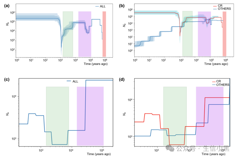
smc++ vcf2smc --missing-cutoff 100000 vcf.gz chr1.smc.gz chr1 CEU:NA12878,NA12879

This means that runs of homozygosity longer than 100,000 bp will be automatically marked as missing data.4Result InterpretationThe first article “Population history and threat identification revealed by population genomic analysis provides insights for the conservation of an endangered maple tree”

• (a): Changes in effective population size (Ne) when all 10 populations are analyzed together.

• (b): Changes in effective population size when populations are divided into two groups (CR and the other 9 populations).

• (c): Population history model when all 10 populations are analyzed together.

• (d): Population history model when populations are divided into two groups (CR and the other 9 populations).

Here, (a) and (b) are results from Stairway Plot 2, while (c) and (d) belong to SMC++ results. These are two different methods for population history inference, each with its advantages and disadvantages.

Interpretation:

① When all 10 populations are included in the analysis, the minimum effective population size (Ne) is estimated to be 188, occurring about 1,000 years ago, while the result obtained from SMC++ is 733, occurring about 8,000 years ago (see figures a, c).

② Stairway Plot 2 (figure a) indicates that after this bottleneck event, Ne has significantly recovered, with the most recent Ne around 210,618. SMC++ (figure c) indicates that the most recent Ne is about 2,256. Both methods also infer that earlier bottleneck events occurred approximately 105,000 years ago (Stairway Plot) and 20,000 years ago (SMC++).

③ When the data is divided into two groups (CR and other populations), the responses of the two groups in the SMC++ model are similar to those of the merged group, with Ne continuously decreasing from the start of the record to the most recent bottleneck event. In this model, the two groups diverged about 170,000 years ago. However, in Stairway Plot 2, although the CR group shows a pattern similar to the merged data (with two significant declines in Ne), the other populations continuously decline in Ne from the start of the record to the present (see figures b, d).

The second article “Large-scale genomics and transcriptomics analysis elucidates the genetic basis of high meat yield in chickens”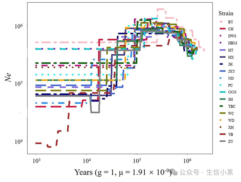Demographic history of 17 local chicken breeds and GGS.The parameter was set generation time (g) = 1, and mutation rate per site (μ) = 1.91 ´ 10^-9. BJY: Beijing You chicken, CH: Chahua chicken, DWS: Daweishan mini chicken, GGS: Gallus gallus spadiceus, HBM: Huaibei Ma chicken, HT: Hetian chicken, HX: Huxu chicken, JH: Jianghan chicken, JXY: Jingxing Yellow chicken, ND: Ningdu chicken, PC: Piao chicken, SH: Sanhuang chicken, TBC: Tibetan chicken, WC: Wenchang chicken, WD: Wuding chicken, XH: Xianghuang chicken, YB: Yuanbao chicken, ZY: Zhengyang chicken.Here, the authors used SMC++ to reconstruct the population history of chickens, specifically analyzing changes in effective population size (Ne) over the past 1,000 to 1,000,000 years. The analysis referenced the study by Nam et al. to obtain model mutation rate (1.91×10⁻⁹) and generation time (1 year).In the figure: GGS represents the wild ancestor chicken, while the others are local chicken breeds.Interpretation:Compared to GGS, all other local chickens show a declining trend, strongly indicating that local chickens have experienced more intense domestication bottlenecks and smaller recent Ne. This demonstrates that domesticated local chickens face greater selective pressure compared to wild chickens.