NPU Neural Processing Unit (7.3) – Quantization Strategy of QAT

Note: Regardless of the quantization method, the ultimate goal is to compress data while minimizing precision loss.

QAT does not quantize a fully trained model, but simulates low-precision behavior while the model weights are still being updated. QAT integrates quantization effects during model training or fine-tuning.

1) Method:

By simulating the effects of low-precision arithmetic during training, the model learns to adjust its weights to minimize the precision loss caused by quantization. This often allows the final quantized model to achieve higher accuracy than applying PTQ on the same original model, especially for aggressive quantization targets.

Figure 1 – QAT Quantization Method

2) Specific Operations:

Simulate quantization and dequantization steps ( FP32→INT8→FP32). These are often referred to as “pseudo-quantization” nodes. During the forward propagation of training, weights and/or activation values are quantized before being used for subsequent operations, and then immediately dequantized. This forces the model to learn parameters that can handle the noise and information loss introduced by the quantization process. This typically results in higher accuracy.

1.Quantization: They receive input floating-point tensors (representing weights or activations) and apply the selected quantization scheme (e.g., mapping floating-point values to the 8-bit integer range using computed scale factors and zero points).

2.Dequantization: After quantization, they immediately convert the low-precision integer representation back to floating-point values using the same scale factors and zero points.

Mathematically, if X is the input floating-point tensor, the pseudo-quantization process x_fq can be represented as:

x_fq=dequantize(quantize(X, scale, zero_point), scale, zero_point)

Here, quantization mapsx to a low-precision range (e.g., INT8), and dequantization maps it back to the floating-point range. The key is that x_fq contains the inherent errors or information loss from the quantization process.

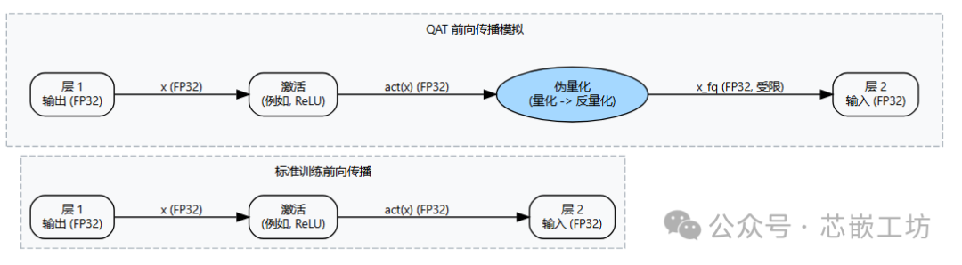
Figure 2 – Comparison of Standard Training and QAT Forward Propagation Process

In QAT, the pseudo-quantization nodes simulate the effects of quantizing the activation values before they are passed to the next layer.

a) Problem:

The core operation in pseudo-quantization is the rounding function, which maps a continuous input range to a discrete set of output values. Mathematically, this function is a step function. A simple rounding function Round(x). Its derivative is zero almost everywhere (on the flat steps) and undefined at the jump points. Standard backpropagation relies on computing gradients to update model weights. If the gradient is zero or undefined, updates cannot be backpropagated through the quantization operation to the previous layers and weights. This effectively hinders the learning process of parameters located before the quantization node. If the gradient is obstructed, how can the model learn to adapt to quantization?

At this point, the Straight-Through Estimator (STE) comes into play. During backpropagation, we need to compute the gradient of the loss L with respect to the input x, represented as ∂L/∂x. Using the chain rule, this is typically computed as:

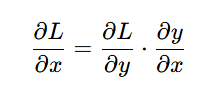
The problem lies in the term, this derivative has issues (mostly zero, undefined at jump points) .

It becomes zero almost everywhere, preventing weight updates.

b) Solution:

The Straight-Through Estimator (STE) provides a practical workaround for this problem. It is an approximation specifically used during backpropagation. The core idea is simple:

1.Forward Propagation: Compute the quantization operation as usual: y=q(x). The quantization effect (precision loss) is fully applied.

2.Backpropagation: When computing the gradient ∂L/∂x, ignore the true derivative of q(x), and instead perform an approximation. The most common STE approximation is to set the gradient ∂y/∂x to 1.

Thus, in backpropagation using STE, the gradient computation becomes:

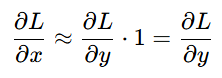
This means that the gradient computed for the output of the quantization node ∂L/∂y is “passed through” to become the gradient for the input ∂L/∂x, as if the quantization operation were an identity function (y=x) used only for gradient computation.

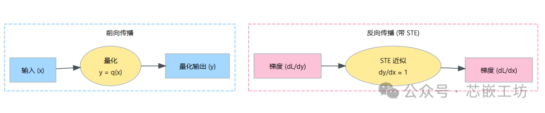
Figure 3 – STE Process

Forward propagation applies actual quantization q(x). Backpropagation uses STE approximation (∂y/∂x≈1), allowing the incoming gradient ∂L/∂y to pass through unchanged, becoming∂L/∂x.

3) QAT vs. PTQ

Feature	Post-Training Quantization (PTQ)	Quantization-Aware Training (QAT)
Main Goal	Speed, simplicity	Maximize accuracy
Accuracy	Generally good, may drop at low bits	Generally higher, especially at low bits
Complexity	Low	High (requires training/fine-tuning)
Computational Cost	Low (calibration + conversion)	High (training/fine-tuning)
Data Requirements	Small calibration set	Full training/fine-tuning dataset
Time	Fast	Slow (training time)
Requirements	Pre-trained model	Training process, data, computational resources
When to Use	First step, sufficient accuracy, limited resources	PTQ is insufficient, aggressive quantization, requires maximum accuracy