Source: DeepHub IMBA


This article is about 4000 words long and is recommended for a reading time of over 10 minutes.
In this article, I will discuss a new semi-supervised, multi-task medical imaging method.
In this article, I will discuss a new semi-supervised, multi-task medical imaging method called Multimix, authored by Ayana Haque (ME), Abdullah-Al-Zubaer Imran, Adam Wang, and Demetri Terzopoulos. This paper was included in ISBI 2021 and presented at the conference in April.
MultiMix performs joint semi-supervised classification and segmentation by adopting a confidence-based augmentation strategy and a novel bridging module that also provides interpretability for multi-tasking. While deep learning models can effectively perform complex image analysis tasks under fully supervised conditions, their performance heavily relies on the availability of large labeled datasets. In the field of medical imaging, manual labeling is not only costly but also time-consuming. Therefore, allowing semi-supervised learning from a limited number of labeled data is considered a solution to the labeling task.
Learning multiple tasks within the same model can further enhance the model’s generalization. Multi-task learning allows for shared representation learning between tasks, requiring fewer parameters and less computation, making the model more efficient and less prone to overfitting.
Extensive experiments were conducted with different amounts of labeled data and multi-source data, demonstrating the effectiveness of their approach. Cross-task intra-domain and cross-domain evaluations were also provided to showcase the model’s potential to adapt to challenging generalization scenarios, which is a critical yet important task for medical imaging methods.
Background Knowledge
In recent years, with the development of deep learning, deep learning-based medical imaging technologies have advanced. However, a fundamental issue with deep learning remains: they require a large amount of labeled data to be effective. This is a bigger problem in the field of medical imaging because collecting large datasets and labeling them is very challenging, as it requires domain expertise, is expensive, time-consuming, and difficult to organize in centralized datasets. Additionally, generalization is also a key issue in medical imaging, as images from different sources can vary significantly both qualitatively and quantitatively, making it difficult to achieve strong performance with a single model across multiple domains. These issues prompted the research of this paper: hoping to address these fundamental problems through some key methods centered on semi-supervised and multi-task learning.
What is Semi-Supervised Learning?
To address the issue of limited labeled data, semi-supervised learning (SSL) has garnered significant attention as a promising alternative method. In semi-supervised learning, unlabelled examples are combined with labeled examples to maximize information gain. There has been extensive research on semi-supervised learning, including general methods and those specific to the medical field. I will not elaborate on these methods, but if you are interested, here is a highlighted list of methods [1,2,3,4].
Another solution to tackle limited sample learning is to use data from multiple sources, as this increases the number of samples and the diversity within the data. However, this approach is challenging as it requires specific training methods; if done correctly, it can be very effective.
What is Multi-Task Learning?
Multi-task learning (MTL) has been shown to improve the generalization capabilities of many models. Multi-task learning is defined as optimizing multiple losses within a single model, accomplished through shared representation learning to complete multiple related tasks. Jointly training multiple tasks within a single model can enhance the model’s generalization since each task influences one another (it is essential to select related tasks). Assuming the training data comes from different distributions, this can be useful for learning in a few supervised ways across limited different tasks. Combining multi-task learning with semi-supervised learning can enhance performance and achieve success in both tasks. Simultaneously completing these two tasks is highly beneficial, as a single deep learning model can perform both tasks very accurately.
Regarding related work in the medical field, specific methods are as follows: [1,2,3,4,5,6,7,8,9,10]. However, the main limitation of these findings is that they did not utilize data from multiple sources, limiting their generalization, and most methods are single-task methods.
Therefore, the paper proposes a new, more general multi-task model, MultiMix, which combines confidence-based bridging blocks to jointly learn diagnostic classification and anatomical structure segmentation from multi-source data. Saliency maps can be generated by visualizing meaningful visual features to analyze model predictions. There are several methods to generate saliency maps, the most significant being calculating the gradient of class scores from the input images. While any deep learning model can be studied for better interpretability through saliency maps, to our knowledge, a saliency bridge between two shared tasks in a single model has not yet been explored.
Algorithm
Let us first define our problem. We train using two datasets, one for segmentation and one for classification. For the segmentation data, we can use symbols XS and Y, representing the images and segmentation masks, respectively. For the classification data, we can use symbols XC and C, representing the images and class labels.
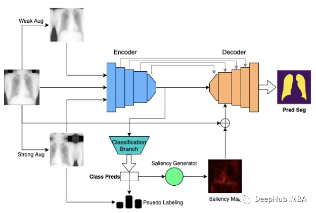
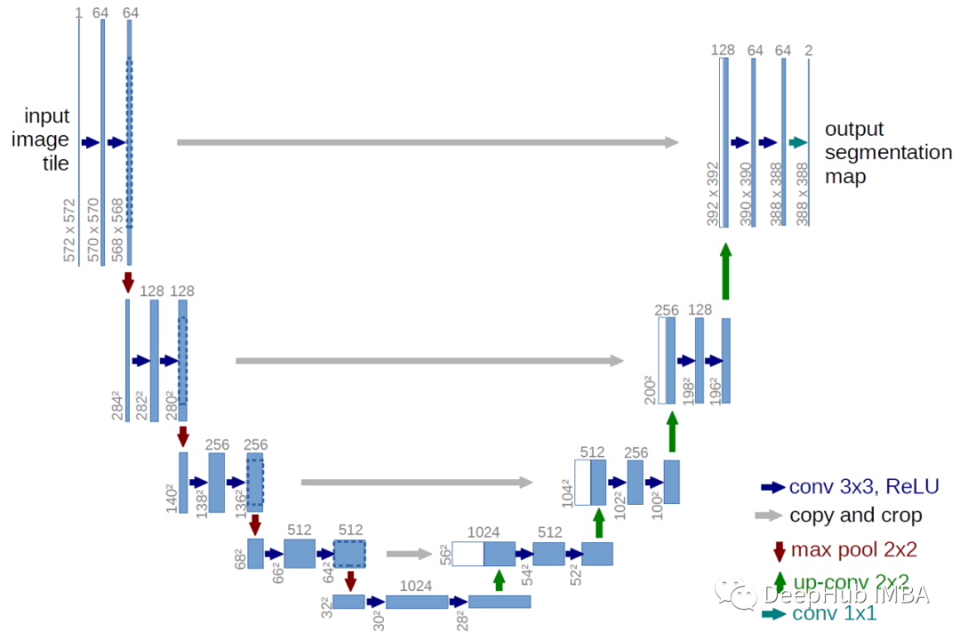
The model architecture uses the baseline U-NET architecture, which is a commonly used segmentation model. The functionality of the encoder is similar to that of a standard CNN. To perform multi-tasking with U-NET, we branch from the encoder and use pooling and fully connected layers to obtain the final classification output.
For the classification method, data augmentation and pseudo-labeling are utilized. Inspired by [1], an unlabelled image is used, and two separate augmentations are performed.
First, the unlabelled image undergoes weak augmentation, and predictions from the model’s current state are designated as pseudo-labels from the weakly augmented version of the image. This is why the method is considered semi-supervised, but we will discuss pseudo-labeling later.
Secondly, the same unlabelled image is strongly augmented, and the loss is computed using both the weakly augmented image and the pseudo-labels from the strongly augmented image itself.
The theoretical basis for such operations is that the model is expected to map the weakly augmented image to the strongly augmented image, thus forcing the model to learn the essential foundational features required for diagnostic classification. Augmenting the image twice also maximizes the potential knowledge gain from the unique image. This also helps improve the model’s generalization, as if the model is forced to learn the most critical parts of the image, it will be able to overcome the differences that arise due to different domains.
The paper uses conventional augmentation methods for weakly augmented images, such as horizontal flipping and slight rotations. The strong augmentation strategy is much more interesting: creating an unconventional, robust augmentation pool and applying a random number of augmentations to any given image. These augmentations are very “extreme,” such as cropping, self-contrast, brightness, contrast, equalization, consistency, rotation, sharpness, shearing, etc. By applying any number of these elements, we can create a very diverse range of images, which is particularly important when dealing with low-sample datasets. We ultimately found that this augmentation strategy is crucial for strong performance.
Now let us revisit the pseudo-labeling process. If the confidence of the model in generating pseudo-labels exceeds a tuned threshold, the image label can prevent the model from learning from incorrect and poor labels. Because when predictions are initially uncertain, the model primarily learns from the labeled data. Gradually, the model becomes more confident in generating labels for unlabelled images, thus becoming more efficient. This is also a very important feature in improving performance.
Now let us look at the loss function. The classification loss can be modeled as follows:
Where L-sub-l is the supervised loss, c-hat-l is the classification prediction, c-l is the label, lambda is the unsupervised classification weight, L-sub-u is the unsupervised loss, c-hat-s is the prediction of the strongly augmented image, and argmax(c-hat-w) is the pseudo-label of the weakly augmented image, with t being the pseudo-label threshold.
This essentially summarizes the classification method; now we continue to the segmentation method.
For segmentation, predictions are made through an encoder-decoder architecture with skip connections, which is quite straightforward. The paper’s main contribution to segmentation is the incorporation of a bridging module to connect the two tasks, as shown in the above figure. Saliency maps are generated based on the classes predicted by the model, using gradients extending from the encoder to the classification branch. The entire process is as shown above, but essentially emphasizes which parts of the images are used by the model to classify pneumonia images.
While we do not know if the segmented images represent pneumonia, the generated maps highlight the lungs. Thus, when using saliency maps to produce and visualize class predictions of images, it is somewhat similar to lung masks. Therefore, we assume that these maps can be used to guide the segmentation in the decoder stage and improve segmentation performance while learning from limited labeled data.
In MultiMix, the generated saliency maps are connected with the input images, downsampled, and added to the feature maps input to the first decoder stage. The connection with the input images can enhance the connection between the two tasks and improve the effectiveness of the bridging module (providing context). Adding both the input images and saliency maps provides more context and information to the decoder, which is crucial when dealing with low-sample data.
Now let’s discuss training and loss. For labeled samples, we typically use the dice loss between the reference lung mask and the predicted segmentation to compute the segmentation loss.
Since we do not have segmentation masks for unlabelled segmentation samples, we cannot directly compute their segmentation loss. Therefore, we calculate the KL divergence between the segmentation predictions of labeled and unlabelled examples. This allows the model to make predictions that are increasingly similar to those from labeled data, enabling the model to fit unlabelled data more appropriately. Although this is an indirect method of calculating loss, it still allows the model to learn a lot from unlabelled segmentation data.
Regarding loss, the segmentation loss can be written as:
Compared to classification, alpha is the reduction weight for segmentation, y-hat-l is the predicted segmentation for labeled data, y-l is the corresponding mask, beta is the unsupervised segmentation weight, and y-hat-u is the unlabelled segmentation prediction.
The model is trained using a combined objective of classification and segmentation losses.
Datasets
The model was trained and tested for classification and segmentation tasks, with data for each task coming from two different sources: a pneumonia detection dataset, which we refer to as Chex [11], and the Japanese Society of Radiological Technology or JSRT [12], used respectively for classification and segmentation.
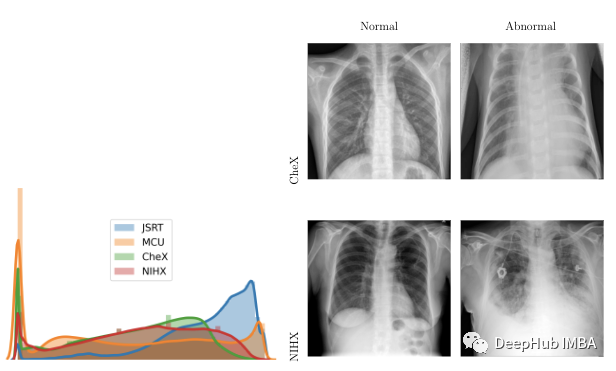
To validate the model, two external datasets were used: the Montgomery County Chest X-ray or MCU [13], and a subset of the NIH Chest X-ray dataset, which we refer to as NIHX [14]. The diversity of sources posed significant challenges to the model, as the quality of images, sizes, ratios of normal to abnormal images, and distribution of intensities across the four datasets varied significantly. The figure below shows the differences in intensity distribution and examples of images from each dataset. All four datasets are licensed under CC BY 4.0.
Results
The paper conducted numerous experiments and utilized different amounts of labeled data across multiple datasets and domains.
Multiple baselines were used in testing, starting with Arale-net and standard classifiers (ENC), which is an encoder extractor with dense layers. We then combined both into a baseline multi-task model (UMTL). Semi-supervised methods (ENCSL), (UMTLS), and a multi-task model with semi-supervised methods (UMTLS-SSL) were also used.
In terms of training, multiple labeled datasets were used. For classification, we used 100, 1000, and all labels, while for segmentation, we used 10, 50, and all labels. For the results, the notation: model – label (e.g., Multimix-10–100) will be used. For evaluation, accuracy (ACC) and F1 scores (F1-N and F1-P) were used for classification, while segmentation utilized DS similarity (DS), JACCARD similarity score (JS), structural similarity index (SSIM), average Hausdorff distance (HD), precision (P), and recall (R).
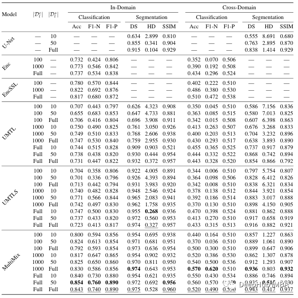 The table shows how the model’s performance improved with the addition of each new component. For the classification task, the confidence-based augmentation method significantly improved performance compared to the baseline model. Multimix-10–100 also outperformed the fully supervised baseline encoder in terms of accuracy. For segmentation, the bridging module produced significant improvements over the baseline U-NET and UMTL models. Even with the lowest segmentation labels, we can see a 30% performance increase, demonstrating the effectiveness of the Multimix model proposed in the paper.
As shown in the table, the performance of MultiMix is also promising in the intra-domain. MultiMix scores better in the classification task across all baseline models. Due to significant differences in the NIHX and CHEX datasets, as mentioned earlier, the scores are not as good as those of the intra-domain model results. However, it does outperform other models.
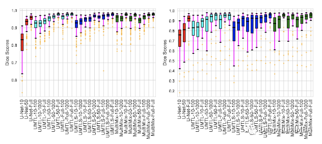
The figure above illustrates the consistency of segmentation results for both intra-domain and cross-domain evaluations. Each image in my dataset shows the dice score of the model. From the figure, it can be seen that compared to the baseline, MultiMix is the strongest model.
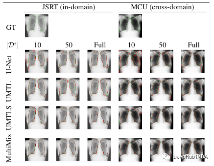
The last figure visualizes the segmentation predictions of the model. The boundaries shown for each proposed segmentation task add a true value comparison against different labeled data. The figure shows a strong consistency between the boundaries predicted by MultiMix and the true boundaries, particularly compared to the baseline. For cross-domain, MultiMix is largely the best, demonstrating strong generalization capabilities.
The table shows how the model’s performance improved with the addition of each new component. For the classification task, the confidence-based augmentation method significantly improved performance compared to the baseline model. Multimix-10–100 also outperformed the fully supervised baseline encoder in terms of accuracy. For segmentation, the bridging module produced significant improvements over the baseline U-NET and UMTL models. Even with the lowest segmentation labels, we can see a 30% performance increase, demonstrating the effectiveness of the Multimix model proposed in the paper.
As shown in the table, the performance of MultiMix is also promising in the intra-domain. MultiMix scores better in the classification task across all baseline models. Due to significant differences in the NIHX and CHEX datasets, as mentioned earlier, the scores are not as good as those of the intra-domain model results. However, it does outperform other models.
The figure above illustrates the consistency of segmentation results for both intra-domain and cross-domain evaluations. Each image in my dataset shows the dice score of the model. From the figure, it can be seen that compared to the baseline, MultiMix is the strongest model.
The last figure visualizes the segmentation predictions of the model. The boundaries shown for each proposed segmentation task add a true value comparison against different labeled data. The figure shows a strong consistency between the boundaries predicted by MultiMix and the true boundaries, particularly compared to the baseline. For cross-domain, MultiMix is largely the best, demonstrating strong generalization capabilities.
Conclusion
In this article, we explained a new sparse supervised multi-task learning model, MultiMix, that can be used for joint learning of classification and segmentation tasks. The paper conducted extensive experiments using four different chest X-ray datasets, demonstrating the effectiveness of MultiMix in both intra-domain and cross-domain evaluations.
The authors of the paper also provided the source code; those interested can check it out:
https://arxiv.org/abs/2010.14731
https://github.com/ayaanzhaque/MultiMix
Editor: Huang Jiyan