MATLAB Basic Practices

• 1. Basic Operations in MATLAB
• 1.1 MATLAB Interface
• 1.2 Common MATLAB Commands
• 1.3 Numerical, Comparison, and Logical Operations
• 1.4 M-files
• 1.5 Live Scripts and Live Editor
• 1.6 Step Signals and Impulse Signals
• 2. MATLAB Plotting
• 2.1 Basic Plotting
• 2.2 Handle Graphics
• 2.3 Interactive Plotting
• some topics
• 3. Time Domain Analysis of Continuous-Time Systems
• 3.1 Introduction
• 3.2 Establishing and Solving Differential Equations

1. Basic Operations in MATLAB

1.1 MATLAB Interface

• Command Window
• Command History
• Workspace
• Editor/Debbuger Window
• Plot Window
• Set Current Path
• Current Path Window

1.2 Common MATLAB Commands

Command	Function	Command	Function
cd	Display or change the working directory	clc	Clear the command window
clear	Clear memory variables	clf	Clear the graphics window
copyfile	Copy files	delete	Delete files or graphic objects
demos	Run example programs	dir, ls	Display files in the current directory
disp	Display variable content	echo	Command window information display switch
load	Load data from a file	movefile	Move files
open	Open a file for editing	pack	Organize memory fragments
pwd	Display the current working path	save	Save variables to a file
type	Display file content	who	Display variables in current memory

Format:

• Query variables: who, whos a*, exist(‘x’)
• Clear variables: clear, clear x, clear a*
• Save and load variables: save, save filename, save filename a, load, load filename

1.3 Numerical, Comparison, and Logical Operations

Using matrices or arrays as basic units

Numerical Operations

Name	Description	Name	Description
+ –	Matrix addition, matrix subtraction	*	Matrix multiplication
/ |Matrix right division, matrix left division	^	Matrix exponentiation
.* .^	Array multiplication, array exponentiation	./ .|Array right division, array left division
‘ .’	Conjugate transpose, transpose	=	Assignment

Comparison and Logic

Name	Description	Name	Description
==	Equal	~=	Not equal
> >=	Greater than, greater than or equal to	< <=	Less than, less than or equal to
&	And	|	Or
~	Not	xor(a,b)	XOR of a and b
any(a)	True if any element in a is non-zero	all(a)	True if all elements in a are non-zero

Numerical Representation and Calculation of Signals

• Numerical representation: represented as a vector in the form of sampled signals
• Numerical computation: description and processing of signals achieved through definitions and operations on vectors and matrices

Example 1.1

% Define time range and step signal
t0=[-5:0.05,5]';% Define time vector
u0=double(t0>0);% Define step signal
%% Define original signal
x0=sin(2*pi*t).*u0;% Define $x(t)=	ext{sin}(2	ext{pi} t)u(t)$
y0=exp(-t0).*u0;% Define $y(t)=e^{-t}u(t)$
tLim=[-1,2]% Set target time interval $[-1,2]$
%% Extract target interval signal
idx=(t0>=tLim(1)&&t0<=tLim(2));% Filter time points in $[-1,2]$
t=t0(idx);% Target time vector
x=x0(idx);
y=y0(idx);% Target interval $x(t),y(t)$
%% Calculate signal operation results
z1=2*x;
z4=x+y;
z5=x.*y;
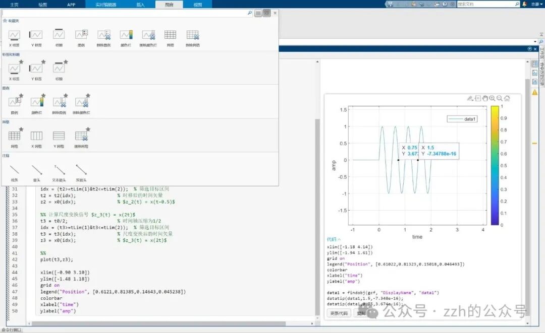
%% Calculate time-shifted signal $z_2(t)=x(t-0.5)$
t2=t0+0.5;% Shift time axis right by 0.5s
idx=(t2>tLim(1)&&t2<tLim(2));% Filter target interval (shifted left by 0.5s)
t2=t2(idx);% Time vector after shift
z2=x0(idx);% Signal after shift
%% Calculate scale-transformed signal $z_3(t)=x(2t)$
t3=t0/2;
idx=(t3>tLim(1)&&t3<tLim(2));% Filter target interval, number of sampling points increased

t3=t3(idx);% Time vector after scale transformation
z3=x0(idx);% Signal after scale transformation

Symbolic Computation

• Define symbolic variables using var=sym(str) or syms var1 var2…
• Symbolic computation is almost identical to numerical computation
• Conversion from symbolic expressions to numerical variables can be done using subs(f,x,y), meaning replace x in the expression with y

Example 1.2 Redo Example 1.1 using symbolic computation

%% Define symbolic variables and signals
syms t x y z1 z2 z3 z4 z5
x=sin(2*pi*t).*heaviside(t);
y=exp(-1*t).*heaviside(t);
%% Calculate signal operation results
z1=2*x;
z2=subs(x,t,t-0.5);
z3=subs(x,t,2.*t);
z4=x+y;
z5=x.*y;

1.4 M-files

Scripts and Functions

Function files can have return values, making them more complex than script files. The first line of a function file declares it as a function file and specifies the function name, parameters, and return values,

function rvalue=functionname(param1,...)

Generally, the function name and the file name of the function file are the same

Program Control Commands

• Sequential execution
• Branching
• if-else-else-end
• switch-case-otherwise-end
• Looping
• for-continue-break-end
• while-continue-break-end
• Error event capture
• try-catch-end

1.5 Live Scripts and Live Editor

• Live Scripts (.mlx) files are MATLAB’s modern programming environment, integrating code, output results, and rich text in one document.
• Advantages over traditional M-files
• Code, results, and explanatory text displayed in the same environment
• Supports mathematical formulas, images, and hyperlinks
• Interactive controls can be added to dynamically adjust parameters
• Supports modular Live Editor Tasks to simplify workflows
• Can be exported in various formats such as PDF, HTML, LaTeX, etc.
• Live Editor Tasks
• Complex operations can be completed without writing code
• Visual parameter adjustments with real-time result viewing
• Automatically generates underlying MATLAB code
• Supports various tasks such as signal processing, data analysis, machine learning, etc.
• Interactive applications embedded in Live Scripts

1.6 Step Signals and Impulse Signals

• heaviside
• dirac

Important Constants and Special Variables in MATLAB

Name	Description	Name	Description
ans	Default variable name for saving results	pi	Pi
eps	Relative error of floating-point numbers	inf	Infinity
NaN,nan	Not a number	i,j	Imaginary unit
realmin,realmax	Minimum/maximum floating-point number	bitmax	Maximum positive integer

2. MATLAB Plotting

• Basic Plotting
• Handle Graphics
• Interactive Plotting

2.1 Basic Plotting

• figure generates a new figure window
• plot, subplot for plotting, plotting in subplots
• hold on/off to turn hold mode on/off
• title to display title
• xlabel, ylabel to display axis labels
• legend to generate legends

Character	Type	Meaning
b/g/r/c/m/y/k	Color	Blue/Green/Red/Cyan/Magenta/Yellow/Black
./x/+/*/s/d/v/^/</>/p/o	Marker Type	Point/X/+/Star/Square/Diamond/Down Triangle/Up Triangle/Left Triangle/Right Triangle/Pentagon/Circle
-/：/-./–	Line Type	Solid Line/Dotted Line/Dash-Dotted Line/Dashed Line

• Plot discrete-time signals using stem
• Plot symbolic functions
• First use the subs function to calculate sampled values at sampling moments, then use the plot function to plot
• A simpler method: ezplot

2.2 Handle Graphics

• Get and modify handle properties
• gcf, gca, gco, gcbf, gcbo to get current… handles
• get, set to access handle properties
• Example
• get(gca)
• set(gca,’XLim’,[0,100])
• get(gca,’XLim’)

Function	Target Object	Typical Application Scenario
<span>gcf</span>	Current figure window	Modify window title, size, color, etc.
<span>gca</span>	Current axes	Adjust axes limits, ticks, labels, etc.
<span>gco</span>	Most recently clicked graphic object	Interactively edit graphic elements (e.g., lines).
<span>gcbf</span>	Window that triggered the callback	Locate the source window in GUI development.
<span>gcbo</span>	Graphic object that triggered the callback	Identify the source control in GUI development.

2.3 Interactive Plotting

• Under the View menu
• Figure Toolbar, Camera Toolbar, Plot Edit Toolbar
• Figure Palette, Plot Browser, Property Editor
• Directly manipulate data in the Workspace
• Output graphics
• Copy Figure
• Save as
• Generate Code

some topics

• Control System Demonstration
• GPU Accelerated Computing
• Cloud Computing and Parallel Computing
• MATLAB vs Python
• LLM-assisted MATLAB Programming

3. Time Domain Analysis of Continuous-Time Systems

3.1 Introduction

• Input-Output Method
• LTI systems can be described using a single high-order differential equation

Example 3.1 Describe the following system

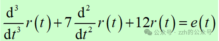
% Define coefficients of the left side of the differential equation (from high to low, fill in missing terms with zero)
a=[1,7,0,12];
% Define coefficients of the right side of the differential equation
b=1;
% Establish continuous-time system transfer function model
sys=tf(b,a);
%b is the numerator polynomial coefficients arranged in descending order of s;
%a is the denominator polynomial coefficients arranged in descending order of s;
%sys is the generated transfer function object (tf type)

• State Variable Description Method
• A single high-order differential equation can be transformed into a system of two multivariable first-order differential equations: state equation and output equation

Example 3.2 Describe the following system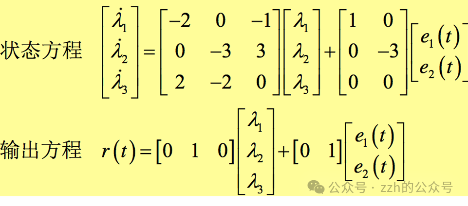

% Define matrices A,B,C,D
A=[-2,0,-1;0,-3,3;2,-2,0];
B=[1,0;0,-3;0,0];
C=[0,1,0];
D=[0,1];
% Establish state equation model
sys=ss(A,B,C,D);

3.2 Establishing and Solving Differential Equations

• The solution of a differential equation includes both the homogeneous solution and the particular solution
• The homogeneous solution is the root of the system characteristic equation, calculated using the roots function.

Example 3.3

% Define characteristic polynomial coefficients
a=[1,7,16,12];
% Find characteristic roots
b=roots(a);

• The particular solution is the output of the system under given signal excitation. Simulated using lsim.

Example 3.4

% Representation of the differential equation
a=[1,2,3];
b=[1,2];
% Establish transfer function model
sys=tf(b,a);
% Set simulation time
t0=[0:0.1:10];
% Define excitation signal 1
e1=t0.*t0;
% Simulate system response
r1=lsim(sys,e1,t0);
% lsim(transfer function, excitation, time)

% Define excitation signal 2
e2=exp(t0);
r2=lsim(sys,e2,t0);

% Plot input-output signals
figure;
% Input
subplot(1,2,1),hold on,box on;
plot(t0,e1,"k-",t0,e2,"k-.");
set(gca,"YScale","log");
set(gca,'Fontsize',16);
legend("e1","e2");
xlabel("Time");
ylabel("Input Signal");

% Output
subplot(1,2,2),hold on,box on;
plot(t0,r1,"k-",t0,r2,"k-.");
set(gca,"YScale","log");
set(gca,'Fontsize',16);
legend("r1","r2");
xlabel("Time");
ylabel("Output Signal");

Knowledge Point 1: Polynomials

polyfun	function
roots	Find the roots of a polynomial
poly	Generate the characteristic polynomial of a matrix or generate polynomial coefficients from polynomial roots
polyval	Return the value of the polynomial at given points
polyvalm	Calculate the value of matrix polynomials
residue	Return the partial fraction expansion of the transfer function, returning values as [residues, poles, direct terms]
polyfit	Least squares polynomial fitting
polyder	Differentiate a polynomial or the product or quotient of two polynomials
polyint	Polynomial integration
conv	Polynomial multiplication
deconv	Polynomial division