1. Prerequisite Knowledge:
1) Python, check online resources (https://www.runoob.com/python/python-tutorial.html or https://colab.research.google.com/).
2) Basic knowledge of mathematics (algebra, probability, calculus), this article introduces basic concepts. For in-depth analysis, continue searching for corresponding online resources. For matters related to AI chips, it is essential to understand the mathematical concepts of the above three subjects.
2. Related Basic Mathematical Concepts:
1) Algebra:
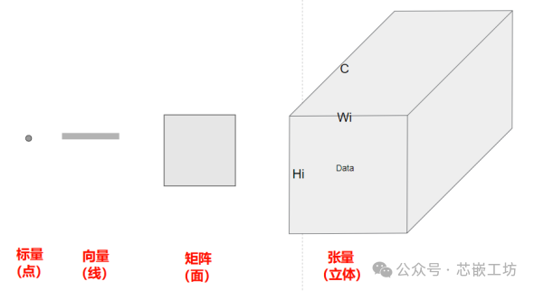
1.1 Scalars (points), vectors (lines), matrices (planes), tensors (volumes)
1.2 Point Multiplication (Element-wise Multiplication):
Multiplying corresponding elements of two matrices, also known as element-wise multiplication. The result is a matrix of the same dimension.
Formula::Cij=Aij×Bij
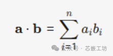
1.3 Dot Product, Vector Inner Product::
The dot product of two vectors of the same length is defined as the sum of the products of their corresponding elements. The result is a single scalar.
Formula::
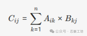
1.4 Matrix Product / Matrix Multiplication:
Each element of matrix C is the dot product of the rows of matrix A and the columns of matrix B (if A is m×n and B is n×p, the result C is m×p).
Formula::
1.5 Norm:
Norm: the “scale” in vector space (vector or matrix).
1.Non-negativity::∥x∥≥0, and ∥x∥=0⟺ x=0 (the zero vector has a unique zero norm).
2.Homogeneity::∥αx∥=∣α∣⋅∥x∥ (where α is a scalar).
3.Triangle Inequality::∥x+y∥≤∥x∥+∥y∥ (the length of the sum of vectors does not exceed the sum of their lengths).
Spaces that satisfy these properties are called Normed Linear Spaces. If only the last two properties are satisfied, they are called Seminorms (which can assign zero length to non-zero vectors).
Vector norms:L1/L2/L∞/Lp norms
Matrix norms:Frobenius norm (F-norm)/Operator norms (1-norm, 2-norm, ∞-norm)
|
Norm Type |
Formula |
Core Features |
Typical Application Scenarios |
|
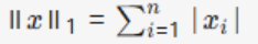
Vector Norm: L1 Norm (Manhattan Norm) |
|
Sum of absolute values, Promotes sparse solutions. |
Feature selection, compressed sensing. Example::x=[2,−3,1], then ||x||1 =6 |
|
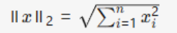
Vector Norm: L2 Norm (Euclidean Norm) |
|
Geometric distance, smooth optimization |
Prevents overfitting in regularization..Example::x=[2,−3,1], then ||x||2 ≈3.74 |
|
Vector Norm: L∞ Norm (Maximum Norm) |
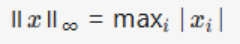 |
Controls maximum value |
Error control. Focus on maximum deviation; used to control worst-case errors (e.g., signal processing)..Example::x=[2,−3,1], then ||x||∞=3 |
|
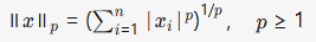
Vector Norm: Lp Norm (Generalized Form) |
 |
|
L1 and L2 are special cases of it (p=1 and p=2). |
|
Matrix Norm:Frobenius Norm (F-norm) |
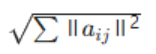 |
Overall measure of matrix elements; Similar to vector L2 norm; measures the overall “size” of all elements in the matrix. |
Low-rank decomposition, matrix approximation. |
|
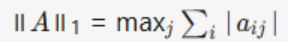
Matrix Norm: Operator1-norm (Column Sum Norm) |
|
Maximum singular value |
Stability analysis |
|
Matrix Norm: Operator2-norm (Spectral Norm) |
 |
Maximum singular value |
Stability analysis |
|
Matrix Norm: Operator∞-norm (Row Sum Norm) |
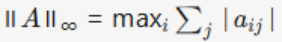 |
Measures the “amplification factor” of the matrix as a linear operator, satisfies compatibility ∥Ax∥≤∥A∥⋅∥x∥ |
|
1.6 Linear Regression (Finding the relationship between input and output):
Linear transformation: the process of converting input data into output predictions, involving a series of linear transformations.
Regression: can model the relationship between one or more independent variables and dependent variables. In the fields of natural and social sciences, regression is commonly used to represent the relationship between inputs and outputs.
Linear Regression: assumes that the relationship between the independent variable x and the dependent variable y is linear, meaning that y is expressed as a weighted sum of the elements in x:
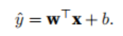
(the vector x corresponds to the features of a single data sample).
The goal of linear regression is to find a set of weight vectors w and a bias b
Classification aims to predict which of a set of categories the data belongs to.
The core objective of the least squares method is to find the best fit between the data and the model by minimizing the sum of squared errors. Given data points (xi,yi) and model function f(x;θ), solve for parameters θ that minimize the sum of squared residuals:
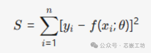
Curve Fitting: (Curve Fitting): Based on discrete data points, select an appropriate function model (e.g., polynomial, exponential function) to construct a continuous curve that describes the relationship between variables..
1.7Loss Function::
Before fitting data with a model, it is necessary to determine a measure of fit.
The loss function can quantify the gap between the actual value and the predicted value of the target.
Typically, we choose non-negative numbers as loss, with smaller values indicating smaller loss, and a perfect prediction has a loss of 0.
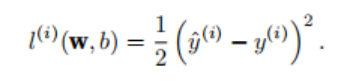
The most commonly used loss function in regression problems is the squared error function.
When the predicted value of sample i is yˆ(i, its corresponding true label is y(i), the squared error can be defined as follows:
2)Calculus(Engine of Learning):
2.1Derivatives (Univariate) and Differentiation:
Calculating derivatives is a key step in the optimization algorithms of deep learning, such as the loss function.
That is, for each parameter, if we increase or decrease the parameter by an infinitesimal amount, we want to know how quickly the loss will increase or decrease.
If the derivative of f exists, this limit is defined as:
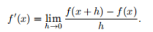
If f ′ (a) exists, then f is said to be differentiable at a; the derivative f ′ (x) is interpreted as the instantaneous rate of change of f with respect to x.
2.2Partial Derivatives (Multivariate):
If the differential of a function of multiple variables,
Let y = f(x1, x2, . . . , xn) is a function with n variables.
The partial derivative of y with respect to the ith parameter xi is:

It can be simply treated as constant (x1, . . . , xi−1,xi+1, . . . , xn as constants (excluding xi), and compute the derivative of y with respect to xi.
2.3Gradient (All Partial Derivatives of Multivariate):
The partial derivatives of a multivariate function with respect to all its variables yield the gradient (gradient) vector.
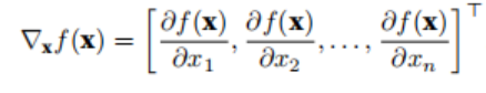
A function f : R n → R has an input of an n dimensional vector x = [x1, x2, . . . , xn] ⊤, and the output is a scalar.
The gradient of the function f(x) with respect to x is a vector containing n partial derivatives:
2.4Chain Rule (Backpropagation):
Multivariate functions are often composite, making it difficult to apply any of the above rules to differentiate these functions. Fortunately, the chain rule can be used to differentiate composite functions.
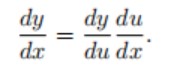
First, consider a univariate function. Suppose the function y = f(u) and u = g(x are both differentiable, according to the chain rule:
Now consider a more general case where the function has an arbitrary number of variables.
Assume the differentiable function y has variables u1,u2,. . . ,um, where each differentiable function ui has variables x1, x2, . . . , xn.
Note that y is a function of x1,x2,…,xn for any i=1,2,…,n, the chain rule gives:
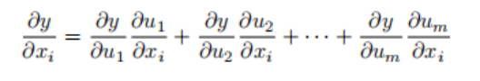
Backpropagation: This algorithm is the core of neural network training. It efficiently computes the gradient of the loss function with respect to each weight in the network using the chain rule of calculus. Then, this gradient is used to update the weights through gradient descent, thereby improving the accuracy of the network.
3)Probability(Handling Uncertainty)
3.1Multiple Random Variables:
3.1.1Joint Probability:
P(A = a, B = b):What is the probability that A = a and B = b occur simultaneously?
3.1.2Conditional Probability:
P(B = b | A = a):A = a has occurred, what is the probability that B = b?
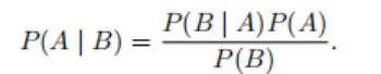
3.1.3Bayes’ Theorem:Multiplication Rule:
Assuming P(B) > 0, solve for one of the conditional variables, obtaining:
3.1.4 Marginalization:Sum Rule:

3.1.5Independence and Dependence::
If two random variables A and B are independent, it means that the occurrence of event A is not related to the occurrence of event B. In this case, statisticians often express this as A ⊥ B. According to Bayes’ theorem, it can also be obtained that P(A | B) = P(A). In other cases, A and B are dependent.
3.1.6Probability Distribution:
Many neural networks use probability distributions to model uncertainty in their predictions. For example, the softmax function can convert the output of the network into a probability distribution over different categories, indicating the confidence of the prediction.
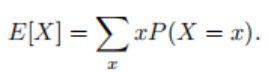
3.2 Expectation and Variance:
To summarize the key features of a probability distribution, some measurement methods are needed. The expectation (or average) of a random variable X is represented as:
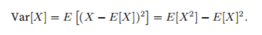
In many cases, we want to measure the bias of the random variable X with respect to its expected value. This can be quantified by variance:
Activation functions (introducing non-linear regression/classification):