Learning PID Control Through Stories and Animations

Advanced Training Course on Optimization and Case Analysis of Continuous Automation Process Design in Pharmaceuticals and Chemicals

Your every share is encouragement for the editor!

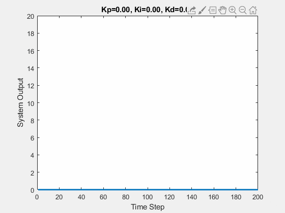
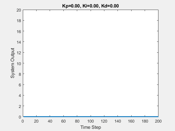
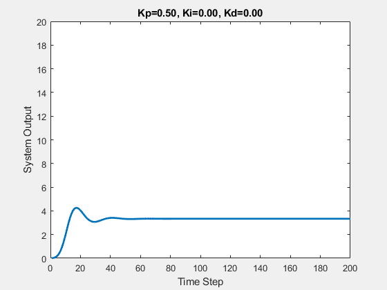
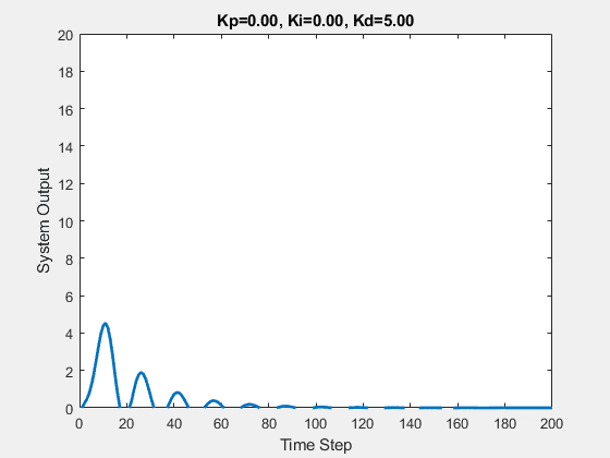
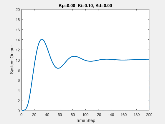
Part One

The initial state of the system is 0, and the target state is 10.

Let’s first demonstrate the process of traversing parameters.

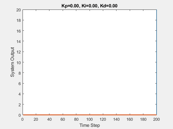
The following animations show the impact of various parameters:

Part Two

Xiao Ming received a task:

There is a water tank that is leaking (and the leak rate may not be constant). The water level must be maintained at a certain position. If the water level is found to be below the required position, water must be added to the tank.

After receiving the task, Xiao Ming kept watch by the tank. After a long time, he got bored and went to read a novel, checking the water level every 30 minutes. The leak was too fast, and every time Xiao Ming checked, the water was almost gone, far from the required height. Xiao Ming changed to checking every 3 minutes, but then he found that the water hardly leaked, and he didn’t need to add water; checking too frequently was futile. After several experiments, he decided to check every 10 minutes. This checking time is called the sampling period.

At first, Xiao Ming used a ladle to add water, but the faucet was over ten meters away from the tank, so he often had to run back and forth several times to add enough water. Then he switched to using a bucket, which allowed him to add a whole bucket at once, reducing the number of trips and speeding up the process. However, several times he overflowed the tank and accidentally got his shoes wet. Xiao Ming then thought of a new method: instead of using a ladle or a bucket, he used a basin. After several tries, he found it just right; he didn’t have to run too many times, nor did he overflow the tank. The size of this water adding tool is called the proportional coefficient.

Xiao Ming also found that although the water wouldn’t overflow, sometimes it would be much higher than the required position, which still posed a risk of wetting his shoes. He then thought of a solution: he installed a funnel on the tank, so that when adding water, he wouldn’t pour it directly into the tank but into the funnel, allowing it to add slowly. This solved the overflow problem, but the water adding speed was now slow, and sometimes it couldn’t keep up with the leak rate. So he tried changing to different sizes of funnels to control the water adding speed, and finally found a satisfactory funnel. The time taken for the funnel is called the integration time.

Xiao Ming finally took a breath, but the task requirements suddenly became stricter; the timeliness of water level control was greatly increased. If the water level was too low, he had to add water to the required position immediately, and it couldn’t be too high, otherwise he wouldn’t get paid. Xiao Ming was troubled again! He thought hard and finally came up with a solution: he kept a basin of backup water nearby. As soon as he noticed the water level was low, he would pour a basin of water in without using the funnel. This ensured timeliness, but sometimes the water level would rise too high. He then drilled a hole just above the required water level and connected a pipe to a lower backup bucket so that the extra water would leak out from the hole above. The speed at which this water leaks out is called the differential time.

After seeing several articles asking about the sampling period, I came up with this story. The analogy of differentiation may be a bit forced, but it helps with understanding.

This is an introductory-level explanation. If it helps beginners understand PID, that would be enough. In the story, Xiao Ming’s experiments are done independently step by step, but in reality, the size of the water adding tool, funnel diameter, and overflow hole size all simultaneously affect the water adding speed and the overshoot, so after doing the subsequent experiments, it often requires modifying the results of the previous experiments.

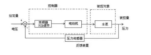
Part Three: Control Model:

A person uses PID control to pour half a cup of water (marked with a scale) from a kettle into a cup and then stops;

Setpoint: the half-cup mark of the cup;

Actual value: the actual water level in the cup;

Output value: the amount poured from the kettle and the amount scooped from the cup;

Measurement sensor: a person’s eyes

Execution object: the person

Positive execution: pouring water

Negative execution: scooping water

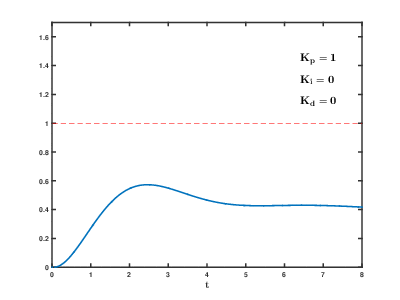
1. P Proportional Control, means that when a person sees that the water level in the cup does not reach the half-cup mark, they pour a certain amount from the kettle into the cup, or if the water level exceeds the mark, they scoop a certain amount out of the cup. This action may cause the cup to be less than half full or more than half full, and then stop.

Note: P proportional control is the simplest form of control. The output of its controller is proportional to the input error signal. When only proportional control is used, the system output has a steady-state error.

2. PI Integral Control, means that the person pours a certain amount into the cup, and if they find that the water level does not reach the mark, they keep pouring. Later, if they find that the water level exceeds half a cup, they scoop some out, and repeat until the water level reaches the mark.

Note: In integral control, the output of the controller is proportional to the integral of the input error signal. If a control system has a steady-state error after reaching steady state, it is called a system with steady-state error. To eliminate steady-state error, an “integral term” must be introduced into the controller. The integral term depends on the time integral of the error, and as time increases, the integral term increases. Thus, even if the error is small, the integral term will increase over time, pushing the controller’s output to further reduce the steady-state error until it equals zero. Therefore, the proportional plus integral (PI) controller can eliminate steady-state error after reaching steady state.

3. PID Differential Control, means that a person’s eyes observe the distance between the water level in the cup and the mark. When the difference is large, they pour a large amount from the kettle. When they see the water level approaching the mark, they reduce the amount poured from the kettle, slowly approaching the mark until stopping. If they can stop precisely at the mark, it is called zero steady-state error; if they stop near the mark, it is called having steady-state error.

Note: In differential control, the output of the controller is proportional to the derivative of the input error signal (i.e., the rate of change of error).

In engineering practice, the most widely used control method is proportional, integral, and differential control, collectively known as PID control or PID regulation. The PID controller has been around for nearly 70 years, and its simple structure, good stability, reliability, and ease of adjustment have made it one of the main technologies in industrial control. When the structure and parameters of the controlled object cannot be fully grasped, or when precise mathematical models cannot be obtained, and other control theory techniques are difficult to apply, the structure and parameters of the system controller must rely on experience and on-site debugging, making PID control technology the most convenient option. That is when we do not fully understand a system and controlled object, or cannot obtain system parameters through effective measurement methods, PID control technology is the most suitable to use. In practice, there are also PI and PD controls. The PID controller calculates the control quantity based on the system error using proportional, integral, and derivative calculations.

Proportional (P) Control

Proportional control is the simplest form of control. The output of its controller is proportional to the input error signal. When only proportional control is used, the system output has a steady-state error.

Integral (I) Control

In integral control, the output of the controller is proportional to the integral of the input error signal. If a control system has a steady-state error after reaching steady state, it is called a system with steady-state error. To eliminate steady-state error, an “integral term” must be introduced into the controller. The integral term depends on the time integral of the error, and as time increases, the integral term increases. Thus, even if the error is small, the integral term will increase over time, pushing the controller’s output to further reduce the steady-state error until it equals zero. Therefore, the proportional plus integral (PI) controller can eliminate steady-state error after reaching steady state.

Derivative (D) Control

In derivative control, the output of the controller is proportional to the derivative of the input error signal (i.e., the rate of change of error). During the adjustment process of the automatic control system to overcome the error, oscillation or even instability may occur. The reason is the presence of large inertial components or delay components, which suppress the error, but their changes always lag behind the change in error. The solution is to make the effect of error suppression change “in advance”, meaning that when the error approaches zero, the effect of error suppression should also be zero. This means that introducing only the “proportional” term in the controller is often not enough; the role of the proportional term is merely to amplify the magnitude of the error, while the current need is to add the “derivative” term, which can predict the trend of error change. Thus, a controller with proportional plus derivative (PD) control can improve the dynamic characteristics of the system during the adjustment process.

When tuning PID parameters, having a theoretical method to determine PID parameters is of course the ideal method, but in practical applications, more often the parameters are determined through trial and error.

Increasing the proportional coefficient P generally speeds up the system’s response, which helps reduce static error in cases with steady-state errors. However, if the proportional coefficient is too large, it can lead to significant overshoot and oscillation, worsening stability.

Increasing the integral time I helps reduce overshoot and oscillation, increasing the system’s stability, but it prolongs the time to eliminate steady-state error.

Increasing the derivative time D helps speed up the system’s response, reduces the overshoot, and increases stability, but it weakens the system’s ability to suppress disturbances.

During testing, one can refer to the above parameters’ influence trends on the system control process and implement the tuning steps of first adjusting proportional, then integral, and finally derivative.

General Methods for Tuning PID Controller Parameters:

Tuning PID controller parameters is the core content of control system design. It determines the proportional coefficient, integral time, and derivative time of the PID controller based on the characteristics of the controlled process. There are many methods for tuning PID controller parameters, broadly categorized into two types:

One is theoretical calculation tuning methods. This mainly relies on the mathematical model of the system to determine controller parameters through theoretical calculations. The data obtained through this method may not be directly usable and must be adjusted and modified through practical engineering;

The second is engineering tuning methods, which mainly rely on engineering experience and are directly conducted during experiments in the control system. These methods are simple and easy to master and are widely used in engineering practice. The engineering tuning methods for PID controller parameters mainly include critical proportional method, reaction curve method, and decay method. Each of these methods has its characteristics, but they all share the common point of being adjusted through experiments and then tuning the controller parameters according to engineering experience formulas. Regardless of which method is used to obtain the controller parameters, they require final adjustments and improvements during actual operation.

Currently, the critical proportional method is generally adopted. The steps for tuning PID controller parameters using this method are as follows:(1) First, pre-select a sufficiently short sampling period to let the system operate; (2) Only add the proportional control element until the system’s step response shows critical oscillation, recording the proportional gain and critical oscillation period at this time; (3) Calculate the PID controller parameters through formulas under certain control conditions.

Setting PID parameters relies on experience and familiarity with the process, tracking measurement values against setpoint curves to adjust the sizes of P, I, and D.

Common Mnemonics from Books:

Find the best parameters from small to large in order;

First proportional, then integral, and finally add derivative;

If the curve oscillates frequently, enlarge the proportional dial;

If the curve drifts around a large bay, turn the proportional dial smaller;

If the curve deviates and recovers slowly, reduce the integral time;

If the curve fluctuates with a long period, increase the integral time;

If the curve oscillates quickly, first reduce the derivative;

If there is a large inertia causing slow fluctuations, increase the derivative time;

The ideal curve has two waves, high before low in a 4:1 ratio;

Observe, adjust, and analyze more, and the quality of regulation will not be low.

In my opinion, the size of PID parameter settings depends on the specific situation of the controlled object; on the other hand, it relies on experience. P addresses amplitude oscillation, and if P is too large, it will result in larger amplitude oscillation but a smaller oscillation frequency, leading to longer stabilization time; I addresses the speed of response, with larger I resulting in slower response speed and vice versa; D eliminates static error, generally set small, and has a minor influence on the system.

How to Best Adjust PID Parameters

(1) Tuning Proportional Control

Gradually increase the proportional control effect, observing each response until a quick response with small overshoot is achieved.

(2) Tuning Integral Element

If the steady-state error cannot meet the requirements under proportional control, integral control needs to be added.

First, reduce the proportional coefficient selected in step (1) to 50-80% of its original value, then set the integral time to a larger value and observe the response curve. Then reduce the integral time, increase the integral effect, and adjust the proportional coefficient accordingly, repeating until a satisfactory response is achieved, determining the parameters for proportional and integral.

(3) Tuning Derivative Element

If after step (2), PI control can only eliminate steady-state error but the dynamic process is unsatisfactory, derivative control should be added to form PID control. First set the derivative time TD=0, gradually increase TD, while adjusting the proportional coefficient and integral time accordingly, repeating until satisfactory control effects and PID parameters are obtained.

Part Three

What is PID?

PID stands for “Proportional, Integral, Derivative” and is a very common control algorithm.

PID has a history of 107 years .

It is not something very sacred; everyone has definitely seen actual applications of PID.

For example, quadcopters, balance cars… also car cruise control, temperature controllers on 3D printers….

In scenarios where a certain physical quantity needs to be “stabilized” (such as maintaining balance, stable temperature, speed, etc.), PID will play a big role.

Now the question arises:

For example, if I want to control a “quick heater” to maintain the temperature of a pot of water at 50℃, such a simple task, why do we need to use the theory of calculus?.

You must be thinking:

Isn’t this so easy? If it’s below 50 degrees, let it heat up; if it’s above 50 degrees, cut off the power. Isn’t it enough? A few lines of code using Arduino can do it in no time.

That’s right! In cases where the requirements are not high, it can indeed be done this way! But! If we change the scenario, you will know where the problem lies:

What if my controlled object is a car?

If I want to keep the car’s speed at 50km/h, would you dare to do it this way?

Imagine this: if the cruise control computer of the car detects a speed of 45km/h at a certain moment, it immediately commands the engine: accelerate!

As a result, the engine suddenly goes to 100% throttle, and the car suddenly accelerates to 60km/h.

At this point, the computer issues a command: brake!

As a result, screech……………wow…………(passengers vomit)

Therefore, in most cases, using “on-off” control for a physical quantity seems relatively simple and crude. Sometimes, it cannot maintain stability. This is because microcontrollers and sensors are not infinitely fast; collecting and controlling take time.

Moreover, the controlled object has inertia. For example, when you unplug a heater, its “residual heat” (i.e., thermal inertia) may still cause the water temperature to continue to rise for a while.

This is when an ‘algorithm’ is needed:

• It can bring the physical quantity that needs to be controlled close to the target.

• It can “foresee” the trend of this quantity’s change.

• It can also eliminate static errors caused by heat dissipation, resistance, and other factors.

• ….

Thus, mathematicians of the time invented this timeless algorithm—this is PID.

You should have already understood that P, I, and D are three different adjustment effects that can be used alone (P, I, D), in pairs (PI, PD), or all together (PID).

What are the differences among these three effects? Please be patient, let me explain slowly.

First, let’s talk about the three basic parameters of the PID controller: kP, kI, kD.

kP

P stands for proportional. Its effect is the most obvious, and the principle is the simplest. Let’s start with this:

The quantity to be controlled, such as water temperature, has its current ‘value’ and our expected ‘target value’.

• When the difference between the two is small, let the heater “lightly heat it up.

• If the temperature drops significantly for some reason, let the heater “apply a little more effort to heat it up.

• If the current temperature is much lower than the target temperature, let the heater “run at full power to quickly bring the water temperature close to the target.

This is the function of P. Compared to on-off control methods, isn’t it much more “gentle”?

When actually writing the program, you establish a linear relationship between the deviation (target minus current) and the adjustment device’s “adjustment strength”, which can achieve the most basic “proportional” control.

The larger kP is, the more aggressive the adjustment action is; if kP is smaller, the adjustment action becomes more conservative.

If you are making a balance car, with the effect of P, you will find that the balance car shakes back and forth around the balance angle, making it difficult to stabilize.

If you have reached this point—congratulations! You are just one small step away from success!

kD

The effect of D is easier to understand, so let’s discuss D before I.

We already have the effect of P. You might notice that just having P alone seems insufficient to keep the balance car upright, and the water temperature control seems shaky, as if the entire system isn’t particularly stable, always “trembling”.

Imagine a spring: it is currently at the balance position. If you pull it and then let go, it will start to oscillate. Because the resistance is small, it may oscillate for a long time before stopping at the balance position.

Now imagine if the system shown above is submerged in water: if you pull it and then let go, the time it takes to stop at the balance position will be much shorter.

We need a control effect that tends to make the controlled physical quantity’s “rate of change” approach zero, similar to a “damping” effect.

Because when approaching the target, the control effect of P becomes smaller. The closer you get to the target, the gentler P’s effect becomes. Many internal or external factors cause small fluctuations in the control quantity.

The role of D is to make the rate of change of the physical quantity approach zero; whenever this quantity has a rate, D applies force in the opposite direction, trying to stop this change.

The larger the kD parameter, the stronger the force applied in the opposite direction to stop the change.

If the balance car has both P and D control effects, if the parameters are adjusted appropriately, it should be able to stand upright~ Let’s cheer!

Wait, it seems that the PID trio has one more member. It looks like PD can keep the physical quantity stable, so why do we need I?

Because we often overlook an important situation:

kI

Let’s take the example of hot water. Suppose a person takes our heating device to a very cold place and starts heating water.They need to heat it to 50℃.

Under the effect of P, the water temperature slowly rises. Until it reaches 45℃, they notice a bad thing: the heat dissipation speed is equal to the heating speed due to the cold weather.

What to do now?

• P thinks: I am close to the target, so I only need to heat it a little.

• D thinks: the heating and heat dissipation are equal, and the temperature is stable. I don’t seem to need to adjust anything.

As a result, the water temperature remains stuck at 45℃, and it never reaches 50℃.

As a person, based on common sense, we know that we should further increase the heating power. But how much should we increase it? How to calculate?

The method devised by earlier scientists is truly ingenious.

Set an integral quantity. As long as there is a deviation, continuously integrate (accumulate) the deviation and reflect it in the adjustment strength.

This way, even if the difference between 45℃ and 50℃ is not large, as time goes on, as long as it has not reached the target temperature, the integral quantity will continue to increase. The system will gradually realize: it has not yet reached the target temperature, and the power needs to be increased!

Once the target temperature is reached, assuming there are no fluctuations, the integral value will stop changing. At this point, the heating power is still equal to the heat dissipation power. However, the temperature remains steadily at 50℃.

The larger the kI value, the greater the coefficient for integration, leading to a more pronounced integral effect.

Therefore, the role of I is to reduce static errors in steady situations, allowing the controlled physical quantity to get as close to the target value as possible.

I also has a problem during use: it requires setting an integral limit to prevent the integral quantity from becoming too large at the beginning of heating, making it difficult to control.

Source: Network

Editor: Chemical Engineer Club

Copyright Statement

Disclaimer: The copyright of the article belongs to the original author. If there are issues regarding the content, copyright, or other matters, please contact us for deletion! The content of the article reflects the author’s personal views and does not represent the views of this public account. This public account reserves the final right of interpretation of this statement.