Introduction to Wigner Distribution
The Wigner distribution is a probability density distribution used in quantum mechanics. It maps quantum states into phase space to describe the probability distribution of quantum systems. It was proposed by Eugene Wigner in 1932 and is primarily used to describe the states of quantum systems, particularly in fields such as quantum optics.
1. Definition of Wigner Distribution
The Wigner distribution is defined by introducing the displacement operator, which represents the distribution of quantum states in phase space. Its mathematical expression is as follows:
Where:
-
( \rho ) is the density matrix of the system.
-
( D(\beta) ) is the displacement operator, defined as:
Where ( a^\dagger ) and ( a ) are the creation and annihilation operators, and ( \beta ) is a complex number representing the coordinates in phase space.
-
( \alpha = x + ip ) is the phase space coordinate, typically represented as ( \alpha = x + ip ).
-
( W(\alpha) ) represents the probability distribution of the quantum state in phase space.
2. Physical Significance of Wigner Distribution
The Wigner distribution is not just a mathematical tool; it also has practical physical significance:
- Correlation: Unlike classical mechanics, quantum states can not only be represented in phase space, but their distribution can also take negative values, indicating the non-classical characteristics of quantum systems.
- Non-negativity: The negative values of the Wigner distribution reflect the non-classicality of quantum states. For example, certain quantum states, such as entangled states, may exhibit negative Wigner distributions.
- Quasi-classicality: In large-scale cases, the Wigner distribution approaches the distribution of classical systems. For instance, for classical thermal states, the Wigner distribution is typically a non-negative Gaussian distribution.
3. Calculation Methods for Wigner Distribution
There are several methods for calculating the Wigner distribution. Below are some commonly used calculation methods:
3.1 Calculation Based on Density Matrix
A common method for calculating the Wigner distribution is through the density matrix to compute its phase space distribution:
3.2 Numerical Method: Lattice Integration Method
Using numerical methods, such as the Monte Carlo method, we can approximate the calculation of the Wigner distribution through lattice integration.
3.3 Empirical Physical Comparison
The Wigner distribution can be used not only for theoretical research of quantum systems but also for comparison with classical physical measurements to verify the properties of quantum systems.
4. High-level Applications of Wigner Distribution
The Wigner distribution is not only used in the study of quantum mechanics but also has various applications. Here are some high-level applications of the Wigner distribution:
4.1 Quantum Optics
The Wigner distribution has important applications in quantum optics, especially in the analysis of the quantum characteristics of photon states.
- Quantum Noise: The Wigner distribution can describe quantum noise, particularly its impact on measurement results in optical experiments.
- Coherence: Through the Wigner distribution of quantum states, we can reveal the coherence and interference effects of quantum states.
4.2 Quantum Computing
In quantum computing, the Wigner distribution can help analyze noise and errors in quantum computation and can further be applied to quantum error correction.
- Feasibility of Quantum Computing: The Wigner distribution serves as a tool for analyzing quantum states in quantum computing, especially playing an important role in complex quantum algorithms.
4.3 Quantum Information and Quantum Communication
The Wigner distribution can also be applied in the fields of quantum information and quantum communication, particularly in the detection of quantum entangled states.
4.4 Quantum Entanglement Analysis in Quantum Computers
The Wigner distribution provides an intuitive representation of quantum states for quantum computers, aiding in the analysis of quantum entanglement and quantum non-locality.
5. Code Example
We will use the Wigner distribution to study quantum entanglement, incorporating W states and decoherence noise models.
5.1 Core Code
% Wigner distribution calculation code: for studying quantum entanglement (including W states and noise models)
% Clear previous variables and figures
clear;
clc;
close all;
% Set parameters
N = 500; % Resolution of phase space
x = linspace(-5, 5, N); % Position coordinate space
p = linspace(-5, 5, N); % Momentum coordinate space
[X, P] = meshgrid(x, p); % Generate 2D grid
% Pauli matrices for quantum bits
sigma_x = [0, 1; 1, 0];
sigma_z = [1, 0; 0, -1];
I = eye(2);
% Generate W state (W-state)
% For 3 quantum bits W state % Corresponding to 3 quantum bits W state (dimension 8)
rho_w = psi_w * psi_w'; % Generate density matrix, dimension should be 8x8
% Calculate noise model (decoherence)
% Here we use a simple decoherence model, such as adding dephasing noise
% Decoherence operation needs to act on each quantum bit
% For a 3 quantum bit system, we need to generate a decoherence operation acting on each quantum bit
noise_op = (1 - dephasing_rate) * I + dephasing_rate * sigma_z; % Decoherence noise operation
% Extend decoherence operation to the entire three quantum bit system
rho_w_noisy = noise_op_3qubit * rho_w * noise_op_3qubit; % Density matrix after decoherence
sigma_x_3qubit = kron(kron(sigma_x, I), I); % Extend sigma_x to three quantum bits operation
% Calculate Wigner distribution
W = zeros(N, N);
for i = 1:N
for j = 1:N
% Define phase space position
x0 = x(i);
p0 = p(j);
% Calculate Wigner function integral
W(i,j) = real(trace(expm(1i * p0 * sigma_x_3qubit) * rho_w_noisy * expm(-1i * x0 * sigma_x_3qubit))); end
end
% Visualize Wigner distribution
figure;
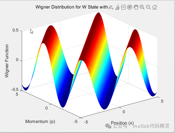
surf(X, P, W);
title('Wigner Distribution for W State with Dephasing Noise');
xlabel('Position (x)');
ylabel('Momentum (p)');
zlabel('Wigner Function');
colormap('jet');
shading interp;
% Add quantum state entanglement analysis
% Measure entanglement: by calculating the purity of the pure state (e.g., using Purity)
purity = trace(rho_w_noisy^2);
disp(['Purity of the system (measure of entanglement): ', num2str(purity)]);
% Calculate entanglement measure (e.g., negative Wigner function value, can be used to confirm entanglement characteristics)
entanglement_measure = min(W(:));
disp(['Entanglement measure (minimum of Wigner distribution): ', num2str(entanglement_measure)]);
% Further analysis (e.g., calculating Von Neumann entropy, etc.)
entropy = -trace(rho_w_noisy * logm(rho_w_noisy));
disp(['Von Neumann Entropy: ', num2str(entropy)]);
5.2 Code Explanation
-
Set Parameters: Initialize the resolution of phase space and position, momentum coordinates.
-
Pauli Matrices for Quantum Bits: Defines the Pauli matrices (\sigma_x, \sigma_y, \sigma_z) and the identity matrix (I), which are important components of quantum bit operations.
-
Generate W State: Constructs the W state for 3 quantum bits to generate the corresponding quantum state vector and calculates its density matrix (\rho_w).
-
Calculate Noise Model (Decoherence): Introduces a decoherence noise model, simulating noise on quantum bits through dephasing operations and calculating the density matrix after decoherence (\rho_w_{\text{noisy}}).
-
Extend Operations to Three Quantum Bits: Extends the Pauli matrix (\sigma_x) and noise operations to the entire three quantum bit system using the Kronecker product.
-
Calculate Wigner Distribution: Calculates the Wigner distribution function at each point using integration.
-
Visualize Wigner Distribution: Displays the Wigner distribution using a surf plot, showing the representation of quantum states in phase space.
-
Entanglement Analysis: Analyzes the entanglement of quantum states by calculating purity, minimum values, etc. Further calculates Von Neumann entropy to assess the entanglement characteristics of the system.
6. Effect Demonstration
7. Access to Complete Code
Visit the following link to access the complete code: https://mbd.pub/o/bread/mbd-aJaZmZlr