Introduction to Python Geographic Analysis: From Beginner to Expert 2 – Geographic Data Processing Made Easy

1Geographic Data Processing

Python Geographic Analysis, from Beginner to Expert Part 2

Python Geographic Remote Sensing Analysis 🌍🐍 (Serial Series) From zero basics to mastery, this series will guide you step by step to master the powerful capabilities of Python in geographic spatial analysis. 🚀 Explore spatial data types, coordinate reference systems, vector operations, and raster operations, and learn to use tools like GeoPandas and Rasterio to process data. 📊 Acquire OSM and census data, delve into remote sensing image processing, band calculations, machine learning predictions, and other advanced skills. 🛰️🌳 Whether you are a beginner or an advanced user, this series will serve as your comprehensive guide to mastering spatial data analysis! 📚

2Spatial Raster Data in Python

The raster data model uses arrays of cells or pixels to represent real-world objects. Raster datasets are commonly used to represent and manage imagery, surface temperatures, digital elevation models, and many other entities.

To process raster data, we will use the rasterio package to convert it into numpy.array. To understand how raster works, we will build a <span>numpy.ndarray</span> from scratch.

Here, we create two objects, one spanning [-90°, 90°] longitude and covering [-90°, 90°] latitude.

import numpy as np
x = np.linspace(-90, 90, 6)
y = np.linspace(90, -90, 6)
X, Y = np.meshgrid(x, y)
X

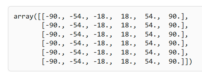
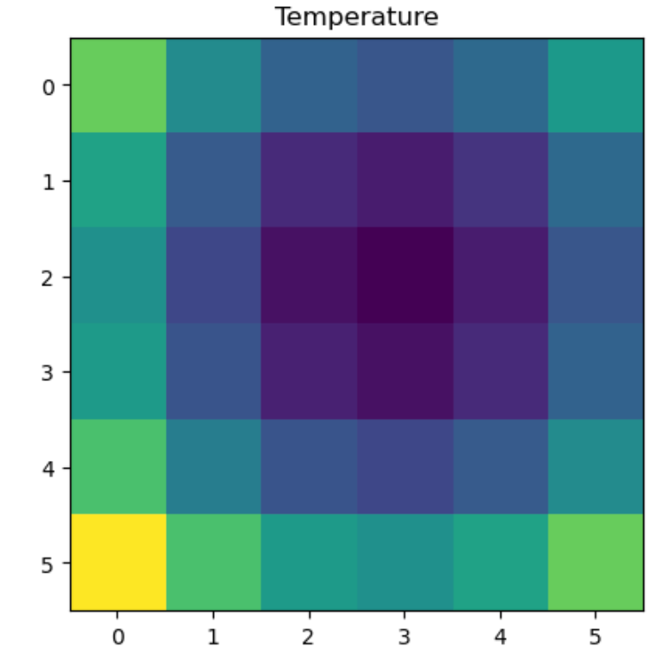
Let’s generate some data representing temperature and store it as an array<span>Z</span>

import matplotlib.pyplot as plt

Z1 =  np.abs(((X - 10) ** 2 + (Y - 10) ** 2) / 1 ** 2)
Z2 =  np.abs(((X + 10) ** 2 + (Y + 10) ** 2) / 2.5 ** 2)
Z =  (Z1 - Z2)

plt.imshow(Z)
plt.title("Temperature")
plt.show()

3Creating Spatial Data TIF from Arrays in Python

We have a data array and some coordinates for each cell, but how do we create a spatial dataset from this? For this, we need three components:

1. Data array, typically xy coordinates
2. A coordinate reference system that defines the coordinate space we are using (e.g., degrees or meters, where the 0° line is, etc.)
3. Transformations defining the upper left corner coordinates and cell resolution

With these components, it only takes a few lines of code to write a valid spatial raster dataset in Python. We just need to provide the information listed above in a format that rasterio can understand.

from rasterio.transform import Affine
import rasterio as rio

res = (x[-1] - x[0]) / 240.0
transform = Affine.translation(x[0] - res / 2, y[0] - res / 2) * Affine.scale(res, res)

# open in 'write' mode, unpack profile info to dst
with rio.open(
    "../temp/new_raster.tif",
    "w",
    driver="GTiff",         # output file type
    height=Z.shape[0],      # shape of array
    width=Z.shape[1],
    count=1,                # number of bands
    dtype=Z.dtype,          # output datatype
    crs="+proj=latlong",    # CRS
    transform=transform,    # location and resolution of upper left cell
) as dst:
    # check for number of bands
    if dst.count == 1:
        # write single band
        dst.write(Z, 1)
    else:
        # write each band individually
        for band in range(len(Z)):
            # write data, band # (starting from 1)
            dst.write(Z[band], band + 1)

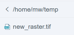
Our new_raster has been successfully written out

Raster data is often “multiband” (e.g., red, green, blue), so I provided code suitable for both multiband and single band data. If you want to store multiband data, the dimensions should be stored as (band, y, x).

4GeoPandas Data Structures

GeoSeries

Similar to a vector, where each entry represents a set of geometries corresponding to a single observation. This can be a single shape (like a single polygon) or may involve multiple shapes forming a single observation.

If you understand Pandas’ DataFrame and corresponding Series, it becomes easy to grasp.

GeoPandas supports three basic types of geometric objects, all of which are well-formed objects:

• Point / MultiPoint
• Line / MultiLine
• Polygon / MultiPolygon

The first example will create a GeoSeries of Points. This can be used to represent individual locations on a map. For example, you could use a point for each location where samples were collected, or to mark cities or other ROIs.

# Point GeoSeries
import geopandas
from shapely.geometry import Point
s = geopandas.GeoSeries([Point(1, 1), Point(2, 2), Point(3, 3)])
s

The next example will create a GeoSeries of Lines. Lines can be used to represent paths of moving objects, routes of roads or rivers, or boundaries between different areas.

# Line GeoSeries
from shapely.geometry import LineString
l = geopandas.GeoSeries([LineString([Point(-77.036873,38.907192), Point(-76.612190,39.290386,), Point(-77.408456,39.412006)])])
l

The final example creates a GeoSeries of Polygons.

# Polygon GeoSeries
from shapely.geometry import Polygon
p = geopandas.GeoSeries([Polygon([Point(-77.036873,38.907192), Point(-76.612190,39.290386,), Point(-77.408456,39.412006)])])
p

GeoDataFrame

A data structure similar to a table that contains a .<span>GeoDataFrame</span>

It has an attribute called “geometry”. Any spatial methods applied to it, or when calling spatial attributes (like area), will act on this “geometry” column.

The “geometry” column can be accessed via the geometry attribute (gdf.geometry) and the name of the geometry column can be retrieved by calling gdf.geometry.name.

Here is an example using the ‘naturalearth_lowres’ dataset. This dataset represents a simplified global country boundary map, which can be used for global scale visualization:

# Load a GeoDataFrame
world = geopandas.read_file(geopandas.datasets.get_path('naturalearth_lowres'))

# Preview the data
world.head()

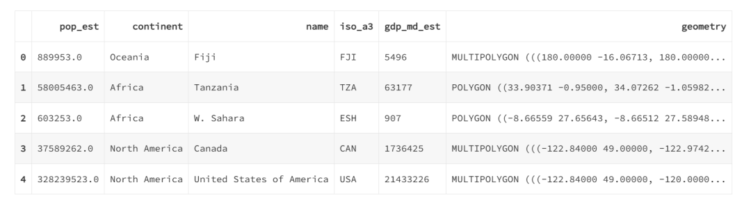
# Plot the GeoDataFrame
world.plot()

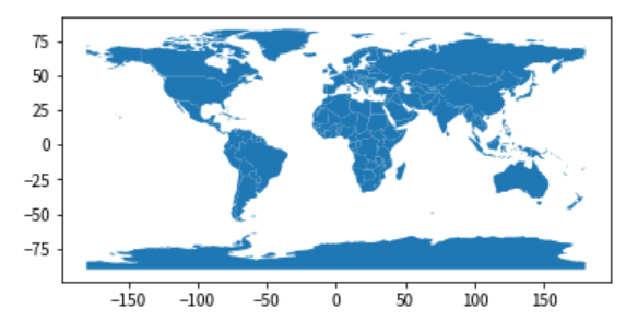
5Spatial Data Processing: Points, Lines, and Polygons in Python

The following code examples are particularly suitable for:

1. Converting files or other data containing coordinates into Shapefiles.
2. Creating and manipulating various spatial objects, including points, lines, and polygons.

Let’s start by importing the necessary modules:

# Import necessary modules first
import pandas as pd
import geopandas as gpd
from shapely.geometry import Point, LineString, Polygon
import fiona
import matplotlib.pyplot as plt
plt.style.use('bmh') # better for plotting geometries vs general plots.

6Creating GeoDataFrame Geometries

The object is a GeoDataFrame with a geometry column used to store spatial data such as points, lines, and polygons. Let’s create an empty column named ‘geometry’ and a new column that will hold our Shapely geometric objects:

# Create an empty geopandas GeoDataFrame
newdata = gpd.GeoDataFrame()
print(newdata)

Functionality requires several key components:<span>GeoDataFrame</span>

• <span>data</span>: pandas DataFrame, dictionary, or an empty list containing the required attribute data.
• <span>crs</span>: The coordinate reference system (CRS) for the geometric objects. This can be any format accepted by <span>pyproj.CRS.from_user_input()</span>
• <span>geometry</span>: The name of the column in the DataFrame used as the geometry or Shapely geometric objects (points, lines, or polygons).

Since Geopandas can handle Shapely geometric objects, we can pass these objects to . This is a particularly useful feature as it allows for easy conversion of text files containing coordinates into Shapefiles.<span>GeoDataFrame</span>

Creating Points from a List of Coordinates

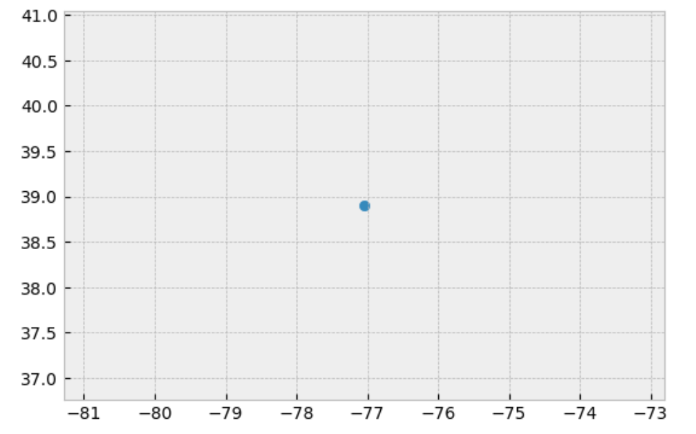
Creating Geopandas point objects from coordinates is very simple. We generate a Shapely point geometry object from a pair of coordinates, create a dictionary containing this geometry and any attributes, and define a coordinate reference system (CRS).

# Coordinates of the GW department of geography in Decimal Degrees
coordinate = [-77.04639494419096,  38.89934963421794]

# Create a Shapely point from a coordinate pair
point_coord = Point(coordinate)

# create a dataframe with needed attributes and required geometry column
df = {'GWU': ['Dept Geography'], 'geometry': [point_coord]}

# Convert shapely object to a geodataframe 
point = gpd.GeoDataFrame(df, geometry='geometry', crs ="EPSG:4326")

# Let's see what we have
point.plot()

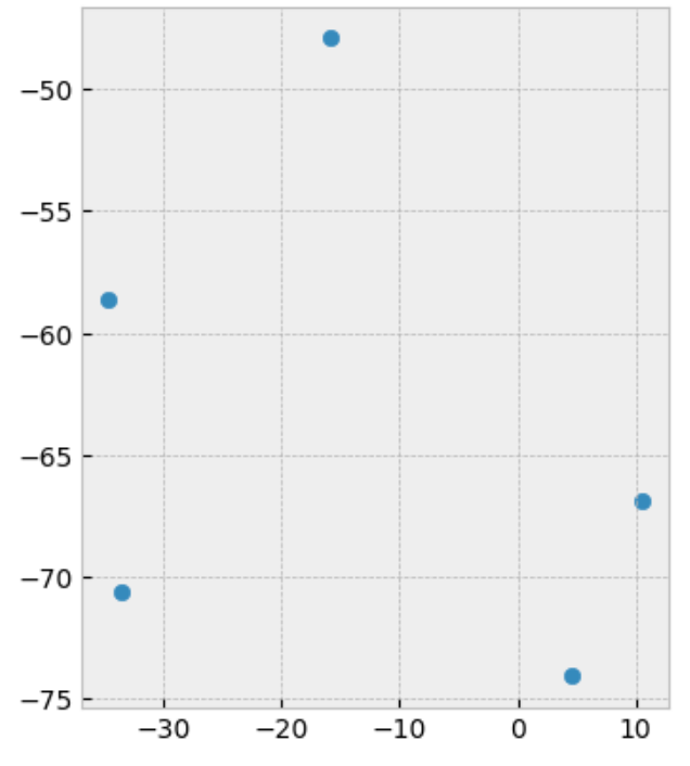
We can also handle a set of points stored in a pandas DataFrame.

# list of attributes and coordinates
df = pd.DataFrame(
    {'City': ['Buenos Aires', 'Brasilia', 'Santiago', 'Bogota', 'Caracas'],
     'Country': ['Argentina', 'Brazil', 'Chile', 'Colombia', 'Venezuela'],
     'lat': [-34.58, -15.78, -33.45, 4.60, 10.48],
     'lon': [-58.66, -47.91, -70.66, -74.08, -66.86]})

# Create Shapely points from the coordinate-tuple list
ply_coord = [Point(x, y) for x, y in zip(df.lat, df.lon)]

# Convert shapely object to a geodataframe with a crs
poly = gpd.GeoDataFrame(df, geometry=ply_coord, crs ="EPSG:4326")

# Let's see what we have
poly.plot()

Creating Points from Latitude and Longitude (Lat, Lon) CSV

A common requirement in spatial data analysis is to create geometric data from CSV files, especially when dealing with large datasets or exporting data from other systems.

Once you learn this code, you won’t have to manually convert many Excel latitude and longitude points into spatial data using ArcGIS.

import pandas as pd
# create an outline of Washington DC and write to CSV
path_to_csv = r'../temp/points.csv'
points = {'Corner':['N','E','S','W'],
          'lon': [-77.0412826538086, -77.11681365966797, -77.01896667480469, -77.0412826538086], 
          'lat': [38.99570671505043, 38.936713143230044, 38.807610542357594, 38.99570671505043]}
points = pd.DataFrame.from_dict(points)
points.to_csv(path_to_csv)              

Then we can read the CSV file and use <span>gpd.points_from_xy()</span> to convert the latitude/longitude values into a list of Shapely Point objects and create a GeoDataFrame.

# read the point data in 
df = pd.read_csv(path_to_csv)

# Create a geodataframe from the data using and 'EPSG' code to assign WGS84 coordinate reference system
points= gpd.GeoDataFrame(df, geometry=gpd.points_from_xy(x=df.lon, y=df.lat), crs = 'EPSG:4326')
points

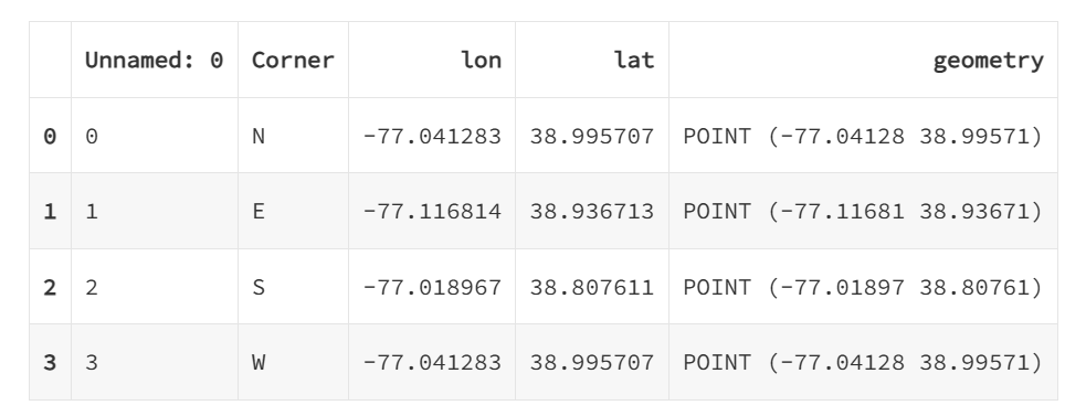
In this case, the <span>points_from_xy()</span> function is used to convert lat and lon into a list of objects. This is then used as the geometry for the GeoDataFrame.

And that’s it for this line of code:

<span>points_from_xy()``shapely.Point``points_from_xy()``[Point(x, y) for x, y in zip(df.lon, df.lat)]</span>

This is a powerful method to quickly convert geographic coordinates stored in CSV format into a spatial format that can be manipulated by Python libraries.

Creating Spatial Lines

Creating lines from points typically represents trajectories or paths in spatial data.

from io import StringIO 
data = """
ID,X,Y,Speed
1,  -87.789,  41.976,  16
1,  -87.482,  41.677,  17
2,  -87.739,  41.876,  16
2,  -87.681,  41.798,  16
2,  -87.599,  41.708,  16
3,  -87.599,  41.908,  17
3,  -87.598,  41.708,  17
3,  -87.643,  41.675,  17
"""
# use StringIO to read in text chunk
df = pd.read_table(StringIO(data), sep=',')

First, we will convert this data into points

#zip the coordinates into a point object and convert to a GeoData Frame
points = [Point(xy) for xy in zip(df.X, df.Y)]
geo_df = gpd.GeoDataFrame(df, geometry=points, crs = 'EPSG:4326')
geo_df.plot()

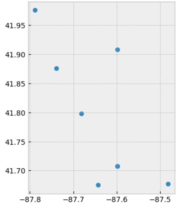
For this, we will group the point data and convert the points into line objects.

# treat each `ID` group of points as a line
lines = geo_df.groupby(['ID'])['geometry'].apply(lambda x:  LineString(x.tolist()))

# store as a GeodataFrame and add 'ID' as a column (currently stored as the 'index')
lines = gpd.GeoDataFrame(lines, geometry='geometry', crs="EPSG:4326") 
lines.reset_index(inplace=True)
lines.plot(column='ID')

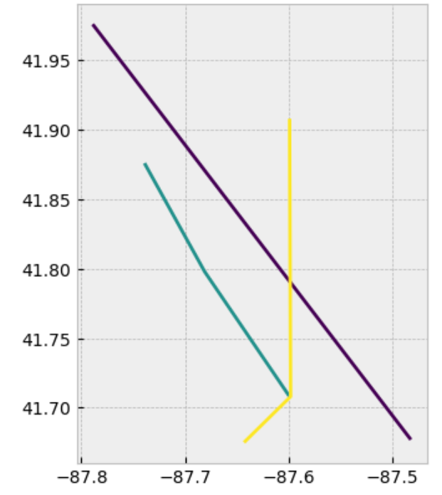
Thus, we see that the paths are treated separately and represented by different lines. And we use<span>ID.plot(column='ID')</span> to plot them.

Constructing Spatial Polygons

The process of constructing polygons in Geopandas is similar to the methods we used earlier for points and lines. The steps are straightforward: we first create a Shapely geometry object from coordinates, integrate this object into a DataFrame with any relevant attributes, and then generate a GeoDataFrame while specifying the appropriate coordinate reference system (CRS).

# Define a list of coordinate pairs
coordinates = [[-77.0412826538086, 38.99570671505043], 
               [-77.11681365966797, 38.936713143230044], 
               [-77.01896667480469, 38.807610542357594],
               [-76.90910339355469, 38.892636142310295]]           

# Construct a Shapely polygon using the list of coordinates
ply_coord = Polygon(coordinates)

# Create a dictionary to hold the necessary attributes and geometry column
df = {'Attribute': ['name1'], 'geometry': [ply_coord]}

# Convert the Shapely object into a Geodataframe and assign a CRS
poly = gpd.GeoDataFrame(df, geometry='geometry', crs="EPSG:4326")

# Visualize the created polygon
poly.plot()

7A Practical Case of Converting a Point to SHP

Since Geopandas integrates with Shapely geometric objects, we can create a shapefile from scratch by feeding Shapely geometric objects into a GeoDataFrame.

This feature is particularly useful as it provides a simple way to convert text files containing coordinates into shapefiles.

Let’s first create an empty GeoDataFrame and add a new column named ‘geometry’ that will contain our Shapely objects:

# Instantiate an empty Geopandas GeoDataFrame
newdata = gpd.GeoDataFrame()

# Add a new column 'geometry' to the GeoDataFrame
newdata['geometry'] = None

print(newdata)

Next, let’s create a Shapely Point that we can later insert into the GeoDataFrame:

# Specify the coordinates for the GWU Department of Geography in Decimal Degrees
coordinates = (-77.04639494419096,  38.89934963421794)

# Create a Shapely point using the coordinates
point = Point(coordinates)

# Display the created point
print(point)

At this point, we have a suitable object.<span>Point</span>

Now we can merge this point into the ‘geometry’ column of the GeoDataFrame:

# Insert the point into the 'geometry' column at index 0
newdata.loc[0, 'geometry'] = point

# Display the updated GeoDataFrame
print(newdata)

Now our GeoDataFrame contains a point that can be exported to a Shapefile.

Let’s further enrich our GeoDataFrame by introducing another column named ‘Location’ with the text ‘GWU Geography’:

# Insert data into a new column 'Location'
newdata.loc[0, 'Location'] = 'GWU Geography'

# Display the updated GeoDataFrame
print(newdata)

Before exporting the data, it’s best to specify the coordinate reference system (CRS, “projection”) for the GeoDataFrame.

The GeoDataFrame has an attribute called crs that represents the coordinate system of the data.

We will assign a CRS to the GeoDataFrame. Fiona is a Python module that has a convenient function called GeoDataFrame for assigning coordinate systems to GeoDataFrames. We will use this function to set the projection to WGS84 (epsg code: 4326), which is the most widely used CRS in the latitude system.

# Assign the GeoDataFrame's CRS to WGS84
newdata.crs = "EPSG:4326"

# Display the GeoDataFrame's CRS
print(newdata.crs)

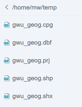
Finally, we can export the data using the function of the GeoDataFrame. This function operates similarly to functions in numpy or pandas, with the only requirement being to provide an output path for the Shapefile:<span>.to_file()</span>

# Specify the output path for the Shapefile
outfp = r"../temp/gwu_geog.shp"

# Export the data to the specified Shapefile
newdata.to_file(outfp)

More Course Recommendations

Hydrology, Water Resources, and Environmental Municipal Courses

1. Mathematical modeling and algorithm applications in smart water management

2. SWMM modeling and LID, retention ponds, river, and water quality simulation applications

3. Secondary development of SWMM based on Python

4. Large-scale watershed modeling based on the VIC distributed hydrological model, runoff case applications, classic paper reproduction, and article writing guidance

5. Typhoon wind field applications and research hotspot analysis based on WRF-LES large eddy simulation, and guidance on article writing ideas

6. Applications of WRF-Hydro in watershed hydrological simulation and analysis of research paper construction ideas

7. SWAT model modeling and case applications

8. HEC-RAS modeling and one-dimensional and two-dimensional simulation applications

9. Hydrus—practical operation techniques and typical case analysis of environmental soil water salt transport models

10. Topics on unsaturated moisture transport, nuclear waste disposal repository nuclide migration, mining well settings and applications, and permeability coefficient evolution based on Tough2 and Toughreact

11. Advanced class in smart water management – deep reinforcement learning control methods and applications for urban drainage systems

12. Research on large eddy simulation based on WRF-LES – teaching, wind field applications, top journal article reproduction, research hotspot analysis, and article writing guidance

13. Case applications of artificial intelligence in the environmental municipal field – real-time control of drainage systems using deep learning as an example

14. SWMM modeling and sponge city, retention pond, river, and water quality quantity simulation applications

Disaster Courses

1. Full process explanation and research paper writing guidance on geological disaster identification, susceptibility assessment, and risk evaluation based on deep learning for regional landslides

Remote Sensing Courses

1. Comprehensive application of ecological environment remote sensing integrating GEE cloud computing platform and Python deep learning

2. Hyperspectral image classification and semantic segmentation based on Pytorch deep learning

3. Specific applications of integrating deep learning and quantitative remote sensing inversion methods in atmospheric environment monitoring – taking aerosol inversion as an example

4. Efficient processing of remote sensing images using R language: advanced training on machine learning, breakpoint detection, and mapping techniques

5. Full process explanation of water quality information extraction, remote sensing inversion, model interpretability, etc., based on machine learning – top journal article reproduction, research hotspot analysis, and research paper writing guidance

6. Inversion of forest canopy height and terrain parameters based on new satellite laser radar – top journal article reproduction, research hotspot analysis, and research paper writing guidance

Ecological Geography Courses

1. InVEST model – water source conservation, habitat quality, soil retention, carbon storage, water quality purification, crop production, ecological services, classic paper explanation reproduction, and article writing

2. CLUE-S model modeling and land use scenario practical exercises

3. DSSAT modeling and simulation of crop growth and development, yield formation processes, future climate scenarios, etc.

4. Species distribution modeling and case analysis based on R language Biomod2

5. Geographic spatial analysis methods and case applications based on ArcGIS and R language

6. Machine learning aiding ecological protection: specific case applications of Biomod2 in species distribution and biodiversity research

7. Comprehensive simulation of ecosystem services under multiple scenarios based on ArcGIS Pro, RULSE, PLUS, and InVEST models

8. Full process teaching of APSIM crop growth model, automated parameter tuning, multi-process batch processing, parameter sensitivity analysis – top journal article reproduction and paper writing guidance

9. Full process explanation of extreme climate index calculation and its impact on vegetation cover change under temporal effects for research paper writing guidance

Atmospheric and Oceanic Courses

1. Construction of FVCOM three-dimensional hydrodynamics and multi-driving force models, Lagrangian particle tracking, tracing, embankments, nesting, and other module applications

2. Establishing localized simulation scheme analysis methods for WRF-CMAQ model

3. Urban-level atmospheric emission inventory production and parsing simulation methods based on Arcgis-Python assisted processing of CAMx-SMOKE

4. Local emission inventory processing methods based on SMOKE model and WRF-SMOKE-CMAQ model case operation

5. WRF meteorological modeling, case applications, and post-processing exquisite mapping

6. EKMA curve plotting and application (OZIPR model)

7. PMF source analysis practical teaching and project application and paper writing training camp based on PMF experimental design

8. Comprehensive teaching of ocean numerical full module depth based on FVCOM-SWAVE and model coupling application practice

9. Modeling methods based on OBM-MCM box model, ozone budget analysis, ozone sensitivity analysis, project business instance explanation, and paper construction idea guidance training

Research Tools Courses

1. Basic calculations and plotting in environmental meteorology and ocean fields using Python

2. NCL data analysis and visualization applications

3. Methods for writing English papers

4. Common case applications of Python in meteorology, ocean, and environmental fields – scientific computing, exquisite plotting, data downloading, etc.