Implementing LLM from Bigram Model with 200 Lines of Python Code

Introduction

The previous article “Implementing LLM from Scratch with 200 Lines of Python” created a “poetry generator” starting from a “probabilistic” implementation, ultimately using PyTorch to realize a classic Bigram model.

In the Bigram model, each character is only related to the previous character. Despite this, our babygpt_v1.py also outputs sentences like “Gradually realizing the path, the spring shirt of the hometown.” which seem quite coherent.

This article continues from babygpt_v1.py, gradually adding mechanisms such as self-attention and positional embedding until a complete GPT is achieved.

Scope and Goals of This Article:

✅ Have read the previous article, can write Python, and have memorized the basic structure of machine learning code;
✅ Attempt to implement a complete language model;
❌ Does not explain mathematical or machine learning principles, only aims for “usability” (because I don’t understand it either);
❌ Does not rely on high-level abstract frameworks, explanations will be provided for the parts used;

Final Effect

Running Method:

$ git clone https://github.com/simpx/buildyourownllm.git
$ cd buildyourownllm
$ pip install -r requirements.txt
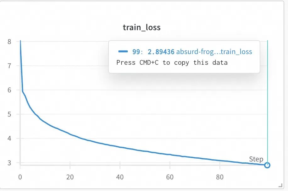
$ python babygpt_v11_hyper_params.py

Results:

step 0: train loss 8.0529, val loss 8.0512, speed: 55304.00 tokens/sec, time: 0m 0.3s
step 50: train loss 5.9337, val loss 6.0072, speed: 102707.49 tokens/sec, time: 0m 8.1s...
step 4950: train loss 2.8944, val loss 3.9963, speed: 104340.95 tokens/sec, time: 12m 57.4s
The spring river water flows like a stream.
Linjiang Fairy by Chen Yunping
The red willows still flutter with butterflies, the Rujiang Bridge. The light gulls cut through the sun as they fly in. Layer upon layer, the soft and sweet is half concealed, the misty dreams return to the man in disarray.
The carriage suddenly arrives, and Xie Xian returns. After all, returning is like a dream, and I will toast and sing again.
A Cut of Plum by Chen Yunping
The peonies are leisurely, the grass is green at first.
---------- In the past, the hate for fame makes tears fall.
A cup of wine is hard to resist. No chance for a bit of grace, a myriad of reds become. And now, I would rather sing and plan, with no way to escape the sorrow.
Linjiang Fairy by Wei Liaoweng
The deep thoughts are hidden, but I am willing to risk injury. The wine often persuades the guests not to linger. The boat is just about to dock, and I must take the easy path to follow. No wind blows my hair.

On my 4090, it takes 12 minutes and 57 seconds to complete training, with the loss values changing as shown in the figure, while on my Mac (16GB memory M1 Pro), the same code took 4 hours to complete training.

Implementing LLM from Bigram Model with 200 Lines of Python Code

Comparison with the words output by the previous Bigram model.

Spring River Moon by Mr. Zhang
The weary traveler. The clear song by the moon's edge, the water plants sing, finishing a cup of wine with the red lotus flowers under the moon, the colorful cage is full of pearls. Only today is ancient. The moon over the creek shines on the guests. Asking for a group, the smoke and waves turn over the ancient half吐, still in the Pengying smoke marsh. The magnolia flower dew bow and knife, let the southeast building be ethereal.

Words output by the Transformer model look significantly more realistic.

Linjiang Fairy by Chen Yunping
The red willows still flutter with butterflies, the Rujiang Bridge. The light gulls cut through the sun as they fly in. Layer upon layer, the soft and sweet is half concealed, the misty dreams return to the man in disarray.
The carriage suddenly arrives, and Xie Xian returns. After all, returning is like a dream, and I will toast and sing again.

After training, our model’s output can clearly show “poetry names” and “people’s names”, this line “The red willows still flutter with butterflies” can almost pass for real.😬

Transformer Model Structure

First, let’s look at the diagram from the “Attention Is All You Need” paper in the “Model Architecture” section. This diagram has been overused, and we will implement the lines and boxes in the diagram step by step.

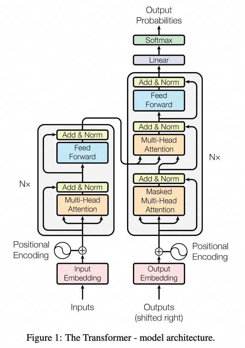
Implementing LLM from Bigram Model with 200 Lines of Python Code

The Transformer was proposed in this paper, initially used to implement translation tasks. The left side of the diagram is the encoder, its Inputs are the “original text to be translated”, which is converted into vectors after computation. The right side of the diagram is the decoder, which is a self-regressive structure. Its input, as shown in the diagram, is the Outputs(shifted right), which is the output from the previous round.

At the beginning of the translation task, the “original text to be translated” is input into the encoder, converted into vectors, while a special token like <sos> (start of sequence) is treated as the initial input for the decoder. Each round of computation in the decoder will incorporate the output from the encoder into some hidden layer. The output of the decoder will serve as the input for the next round of the decoder, repeating this process until the decoder outputs a special token like <eos> (end of sequence), indicating the end.

This structure realizes the association between the “original text to be translated” and the “target text”, and also allows for semantic relationships between the “target text” itself.

Understanding this structure is crucial because today’s large language models are based on the decoder part of the Transformer architecture (hence often referred to as “Decoder-only” architecture). In reality, GPT does not know what “input” or “output” is, nor does it know which part is “human questions” and which part is “AI answers”. In the “Decoder-only” Transformer architecture, each token is equal, and the AI is merely continuously autoregressively “continuing” the text, just like the final effect shown.

It seems that the model outputs the poetry name “Linjiang Fairy” and the person’s name “Chen Yunping”, but in reality, the model is just adding a space after “Linjiang Fairy”, making the reader think it really knows what a “poetry name” is.

For AI, the “dialogue” between humans and AI is just a bunch of tokens separated by line breaks, and only when humans “read” this text do they feel that “it seems like humans and AI are having a dialogue” — the “meaning” is actually assigned by the reader.

Implementing Positional Encoding

In the past, when publishing papers in the systems field, the architecture diagrams were usually “schematic diagrams”, which still had a gap from the real structure. The first time I read a machine learning paper closely, I found that this diagram is actually “code”. Let’s see how to implement the Positional Encoding.

<img alt="Implementing LLM from Bigram Model with 200 Lines of Python Code" src="https://boardor.com/wp-content/uploads/2025/10/05aaa03b-32ec-4df2-94bf-e0a5adc1eaea.jpg"/>

In the original “Attention” paper, a method of “sine-cosine positional encoding” was used, but in fact, GPT uses a simpler method of “learned position embeddings”, as described in the paper “Improving Language Understanding by Generative Pre-Training”.

We used learned position embeddings instead of the sinusoidal version proposed in the original work. We use the ftfy library to clean the raw text in BooksCorpus, standardize some punctuation and whitespace, and use the spaCy tokenizer.

For now, you can ignore the obscure term “learned position embeddings” and directly look at the code implementation (the following is a diff based on babygpt_v1.py, only 9 lines were added, the complete code can be found in babygpt_v2_position.py[1].

class BabyGPT(nn.Module):
-    def __init__(self, vocab_size: int, n_embd: int):
+    def __init__(self, vocab_size: int, block_size: int, n_embd: int):
        super().__init__()
+        self.block_size = block_size
        self.token_embedding_table = nn.Embedding(vocab_size, n_embd)
+        self.postion_embedding_table = nn.Embedding(block_size, n_embd) # Build a "position" mapping
        self.lm_head = nn.Linear(n_embd, vocab_size)
    def forward(self, idx, targets=None):
+        B, T = idx.shape # B is batch size, T is block size
        T = min(T, self.block_size)
        idx = idx[:, -T:] # Regardless of how long the input sequence is, we only take the last block_size tokens
        tok_emb = self.token_embedding_table(idx) # Get the embedding representation of the tokens (B,T,n_embd)
-        logits = self.lm_head(tok_emb)
+        pos_emb = self.postion_embedding_table(torch.arange(T, device=idx.device)) # Get the embedding representation of the positions (T,n_embd)
+        x = tok_emb + pos_emb # Add the positional embedding to the token embedding, x now has "positional" information!
+        logits = self.lm_head(x) # Through the linear layer, remap the embedding results back to vocab_size dimensional space (B,T,vocab_size)

It just works!

As you can see, just 5-6 lines of effective code added a layer to our neural network, allowing our neural network to consider not only the tokens themselves but also the positions of the tokens during training. It’s that amazing.

After all, this is the first time we are “adding a layer”, so let’s carefully interpret the code here.

Line 8: As described by OpenAI, we used a “learnable position embedding matrix” here. In simple terms, we added many parameters, so when the block_size length tokens are input, in addition to obtaining their vectors using the token_embedding_table, we also convert their “positions” into vectors. This conversion table will also be trained in the neural network.
Line 12 ~ 14: Since our postion_embedding_table is a table with keys only of block_size size, regardless of how long the sequence is input, we must truncate it to keep the last block_size tokens.
Line 17: Obtain the vector of the “position” of the tokens, torch.arange(T) actually returns [0,1,2,...,T-1], which is the “position” of each token (isn’t it quite simple?).
Line 18: Add the original token vector and its position vector to form a new vector. At this point, looking back at the Transformer architecture diagram, there is a clear plus sign connecting the “Output Embedding” and “Positional Encoding” nodes, which is not just for aesthetics, but is indeed an “addition”.😄

Other training and inference codes remain unchanged, and we have completed the “positional embedding”. By running python babygpt_v2_position.py, we can see the results, which actually do not show any significant improvement compared to the previous version.

When we modify the model, what exactly did we change?

So far, we have successfully added a layer to the model, which is surprisingly simple. What exactly did we do?

Since this series is “zero-based”, only seeking to use and simply modify the model, we will only attempt to “taste” what we have done.

When we assign a value to another class that also inherits from nn.Module in the constructor of the BabyGPT class, through variable assignment, PyTorch will secretly record all the information. When we later train the model through:

optimizer = torch.optim.AdamW(model.parameters(), lr=learning_rate)

the optimizer will know which layers’ parameters to modify — thus, the parameters of the position embedding we just added are magically “trained”.

When we first execute token embedding (Line 15 of the above code), we obtain a tensor of shape (B, T, n_embd), where B is the batch size, T is the block size, and each token has n_embd parameters, which are floating-point numbers. After executing position embedding (Line 17 of the above code), we obtain a tensor of shape (T, n_embd), which can simply be considered as T * n_embd floating-point numbers.

When the two tensors are added together, we obtain a tensor of shape (B, T, n_embd), but each floating-point number has slightly “increased” a bit, that bit being the numerical representation of the positional information.

As someone without a machine learning background, I feel that the essence of machine learning is — it seems to encode the information we artificially deem necessary into some trainable parameters in various ways. As for “why use addition here?” and “why can the position and token vectors be added, what are their units?” these are not very important. The key point is that “after the addition, the information is not lost” and “the parameters are trainable”.

Always remember, the “model” we see today is all artificially defined. Machine learning is very different from the “precise expression” we usually write in code. In machine learning, the only truly correct method is “iterating and finding ways to reduce the loss value”, not the “model” or the method of “expressing relationships”.😄

The reason for explaining so much here is to avoid students like me, who come from a systems coding background, from getting too entangled in the principles involved.

Implementing Single Head Self-Attention

Finally, we are going to implement the Attention mechanism.🥹

What exactly is Attention? Many articles compare it to how a person focuses on the prominent parts of a photo, which is attention — but why does a machine have “attention”?

When I tried to understand the attention mechanism, I was confused by many “metaphors”. Some said q represents the “current query”, and kv represents other information. Here, I will try to show the specific process to explain how to calculate attention. For readers, the key is to constantly recall the “information” and “shape” represented by the tensors.

From the previous positional encoding, the most important knowledge learned is — “when two numbers are added together, they create a relationship”. Using their sum for subsequent calculations transmits the “information” they each represent.

The Bigram model in the previous article believes that each token is only related to the “previous” token, while the attention mechanism believes that the probability of each token depends on the information of all previous tokens.

The simplest “attention”, weighted summation

Assuming we have a basic “token – feature” matrix v, with a shape of (3, 2), as follows:

>>> v = torch.randint(0, 10, (3, 2)).float()
tensor([[5., 0.], # Token1's features: [FeatureA=5, FeatureB=0]
        [8., 1.], # Token2's features: [FeatureA=8, FeatureB=1]
        [6., 1.]]) # Token3's features: [FeatureA=6, FeatureB=1]

According to the implementation in babygpt_v2_position.py, we can also treat v as the result after embedding the tokens, viewing v as a tensor with batch_size of 1, block_size of 3, and n_embed (the “features” of each token) being a tensor of 2.

How can we calculate a new “token – feature” matrix v2, keeping its shape as (3, 2), but with its content being the feature values of the corresponding position token, plus the average of the feature values of all previous tokens?

We could implement this by traversing, summing, and averaging — but we will use a more “machine learning” approach.

First, calculate a “weight matrix” wei:

>>> tril = torch.tril(torch.ones(3, 3))
tensor([[1., 0., 0.],
        [1., 1., 0.],
        [1., 1., 1.]])
>>> wei = tril / torch.sum(tril, 1, keepdim=True)
tensor([[1.0000, 0.0000, 0.0000],
        [0.5000, 0.5000, 0.0000],
        [0.3333, 0.3333, 0.3333]])

tril is a “lower triangular” matrix of shape (3, 3), functioning similarly to a mask. After dividing this matrix by the sum of each row, we obtain the wei weight matrix, which indicates “how much weight to pay attention to other tokens”. In fact, this is what we call the “attention matrix” — the values here represent the “size of attention” between tokens.

Here’s a more intuitive explanation:

[[1.0, 0.0, 0.0],   # Token1 only focuses on itself
 [0.5, 0.5, 0.0],   # Token2 averages attention on Token1 and Token2
 [0.3333, 0.3333, 0.3333]]     # Token3 averages attention on all tokens

Finally, we perform a simple matrix multiplication to obtain our v2.

>>> v2 = wei @ v
tensor([[5.0000, 0.0000],
        [6.5000, 0.5000],
        [6.3333, 0.6667]])

We can see that each row of the result corresponds to the weighted sum of the columns of v, with the weights determined by the corresponding rows of wei, as explained below.

[[5.0, 0.0],   # Token1's new features: directly retains its own features (weights [1,0,0])
 [6.5, 0.5],   # Token2's new features: average of Token1 and Token2 (weights [0.5,0.5,0])
 [6.333,0.666] # Token3's new features: average of all tokens (weights [1/3,1/3,1/3])]

v2 contains each row corresponding to the new values of the respective token calculated through the “attention” mechanism, which can be used for subsequent predictions of the corresponding token‘s next value, just like the output of the Bigram model.

Notably, in machine learning, there are more elegant ways to obtain wei, but due to space constraints, we won’t elaborate, just familiarize yourself with it.

Another way to calculate wei:

>>> tril = torch.tril(torch.ones(3, 3))
>>> wei = torch.zeros((3, 3))
>>> wei = wei.masked_fill(tril == 0, float('-inf'))
>>> wei = F.softmax(wei, dim=-1)
tensor([[1.0000, 0.0000, 0.0000],
        [0.5000, 0.5000, 0.0000],
        [0.3333, 0.3333, 0.3333]])

Real Attention Calculation, QKV!

In the “Attention” paper, attention calculation requires three matrices. We won’t delve into the reasons, just implement the algorithm directly.

We will take batch_size of 8 and n_embed of 16 as an example to demonstrate the calculation process and results.

Here we use the concept of head, which I personally understand as a “measure word” for the attention mechanism. One head represents a group of QKV calculations.

Step 1: Initialize Input

>>> head_size = 16 # Artificially defined attention dimension
>>> x = torch.randn(1, 8, 16)  # Single batch (B=1), 8 tokens, each token has 16-dimensional features
>>> B, T, C = x.shape  # B=1, T=8, C=16

At this point, x:

          x (1,8,16)
        ┌───────────────────┐
        │ token1 (16 dimensions)      │
        │ token2            │
        │ ...               │
        │ token8           │
        └───────────────────┘

Step 2: Calculate Key/Query/Value

>>> key = nn.Linear(C, head_size, bias=False)
>>> query = nn.Linear(C, head_size, bias=False)
>>> value = nn.Linear(C, head_size, bias=False)
>>> k = key(x)   # (1,8,16)
>>> q = query(x) # (1,8,16)
>>> v = value(x) # (1,8,16)

Key/Query/Value are essentially three linear layers without bias, meaning they each only have one w parameter, which is very simple.

The shapes of the results of the three matrices are the same.

        q/k/v (1,8,16)
        ┌───────────────────┐
        │ New feature1 (16 dimensions)     │
        │ New feature2           │
        │ ...               │
        │ New feature8           │
        └───────────────────┘

Step 3: Calculate Attention Scores (Q·Kᵀ) and Scale

k.transpose(-2, -1) is the transpose of K (changing its shape) so that it can perform matrix multiplication with q. By scaling, we can bring the results to a reasonable range, avoiding gradient vanishing issues.

>>> d_k = k.size(-1)  # Dimension of Key (16)
>>> wei = q @ k.transpose(-2, -1)  # (1,8,8)
>>> wei = wei / (d_k ** 0.5) # (1,8,8)

This is our “attention matrix”!😎 Remember that the previous version of wei was a simple lower triangular matrix, while this one is much more complex.

        q (8,16)           kᵀ (16,8)
        ┌─────────┐        ┌─────────┐
        │ ...     │        │ ...     │
        └─────────┘        └─────────┘
              ↓                ↓
              [[q1·k1, q1·k2, ..., q1·k8],
               [q2·k1, q2·k2, ..., q2·k8],
               ...
               [q8·k1, q8·k2, ..., q8·k8]]
              ↓
              wei (8,8) Each element is a dot product score

Step 4: Apply Mask

tril = torch.tril(torch.ones(T, T))  # Lower triangular matrix
wei = wei.masked_fill(tril == 0, float('-inf'))  # Only keep the current token and previous information

Mask effect:

Original wei:[[ q1·k1, q1·k2, q1·k3, ..., q1·k8 ]
 [ q2·k1, q2·k2, q2·k3, ..., q2·k8 ]
 ...
 [ q8·k1, q8·k2, q8·k3, ..., q8·k8 ]]
After applying the lower triangular mask:[[ q1·k1, -inf,   -inf, ..., -inf  ]
 [ q2·k1, q2·k2, -inf, ..., -inf  ]
 ...
 [ q8·k1, q8·k2, q8·k3, ..., q8·k8 ]]

Step 5: Softmax Normalization

wei = F.softmax(wei, dim=-1)  # Normalize along the last dimension

Example of effect (values are illustrative):

[[1.0, 0.0, 0.0, ..., 0.0]   # token1 can only see itself
 [0.3, 0.7, 0.0, ..., 0.0]   # token2 sees token1 and 2
 ...
 [0.1, 0.1, 0.1, ..., 0.6]]  # token8 sees all history

Step 6: Aggregate Value

out = wei @ v  # (1,8,16)

In out, the output of each token is the weighted sum of the v vectors, with weights coming from the wei representing attention. For example:

out[2] = 0.3*v1 + 0.7*v2 + 0*v3 + ... + 0*v8

Final output result:

        out (1,8,16)
        ┌───────────────────┐
        │ New token1 (16 dimensions)    │  # Contains only token 1 information
        │ New token2          │  # Contains information from token 1 and 2
        │ ...               │  # ...
        │ New token8          │   # Contains information from token 1 ~ 8
        └───────────────────┘

Summary & kvcache

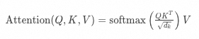
This is the method of calculating attention. Now, looking back at the formulas in the paper, they don’t seem so unfamiliar anymore:

Where:

is the query matrix, dimension , n is the number of queries;
is the key matrix, dimension , m is the number of keys;
is the value matrix, dimension , m is the number of values (same as the number of keys);
is the dimension of keys and queries;
is the scaling factor used to prevent the dot product from being too large, leading to gradient vanishing;

We have implemented the complete formula, and based on the obtained out tensor, we can predict the “next token”, for example, out[1] is calculated using the information from token1 ~ 2 to predict token3. If we are training, we will calculate the out value for each token, and if we are inferring, we only need to incrementally calculate the last out value.

Additionally, by observing the results of the attention score calculation in “Step 2” for the wei matrix:

       q (8,16)           kᵀ (16,8)
        ┌─────────┐        ┌─────────┐
        │ ...     │        │ ...     │
        └─────────┘        └─────────┘
              ↓                ↓
              [[q1·k1, q1·k2, ..., q1·k8],
               [q2·k1, q2·k2, ..., q2·k8],
               ...
               [q8·k1, q8·k2, ..., q8·k8]]
              ↓
              wei (8,8) Each element is a dot product score

We can see that the result of the last row [q8·k1, q8·k2, ..., q8·k8] is only related to q8, but is related to all k1 ~ k8, thus we can conclude that during inference, we only need to calculate the current token’s q, but we still need to calculate the values of all tokens’ k and v — this is why we can use “kvcache” to improve inference performance, while there is no “q-cache” concept.

Attention Code Implementation

In fact, the amount of code is not much, see the complete code in babygpt_v3_self_attention.py, below is the attention part of the code:

class Head(nn.Module):
    def __init__(self, head_size):
        super().__init__()
        self.key = nn.Linear(n_embed, head_size, bias=False)
        self.query = nn.Linear(n_embed, head_size, bias=False)
        self.value = nn.Linear(n_embed, head_size, bias=False)
        self.register_buffer('tril', torch.tril(torch.ones(block_size, block_size)))
    def forward(self, x):
        B, T, C = x.shape # (batch_size, block_size, n_embed)
        k = self.key(x)   # (B, T, head_size)
        q = self.query(x) # (B, T, head_size)
        v = self.value(x) # (B, T, head_size)
        wei = q @ k.transpose(-2, -1) / (k.size(-1) ** 0.5)
        wei = wei.masked_fill(self.tril[:T, :T] == 0, float('-inf'))
        wei = F.softmax(wei, dim=-1) # (B, T, T)
        out = wei @ v # (B, T, T) @ (B, T, head_size) = (B, T, head_size)
        return out

@@ -52,6 +73,7 @@ class BabyGPT(nn.Module):
        tok_emb = self.token_embedding_table(idx) # Get the embedding representation of the tokens (B,T,n_embd)
        pos_emb = self.postion_embedding_table(torch.arange(T, device=idx.device)) # Get the embedding representation of the positions (T,n_embd)
        x = tok_emb + pos_emb # Add the positional embedding to the token embedding, x now has "positional" information!
+        x = self.sa_head(x) # self-attention

As you can see, the implementation is the same as the explanation above. It’s that simple, and we’ve added another layer to our model. After running, you will find that there is still no significant improvement.😅

Implementing the Remaining Layers

So far, we have understood that adding layers to a neural network is simply the process of “adding a new nn.Module” and “applying the new layer in forward”.

Moreover, we have implemented the most important Attention mechanism of the Transformer, and other implementations are common mechanisms in neural networks. Therefore, I will not explain the principles of each subsequent layer in detail, but will briefly introduce their purposes, and through the babygpt_vN_xx.py files, you can see the entire process of adding them. By running the diff command locally to view the differences between two adjacent files, you can understand what has been added.

Although this may seem a bit dubious, who says we are a “zero-based” tutorial?😅

1. Multi-Head Self-Attention

The code can be found in babygpt_v4_multihead_attention.py

In fact, multi-head is just a concat operation on multiple heads, as follows:

+class MultiHeadAttention(nn.Module):
+    def __init__(self, num_heads, head_size):
+        super().__init__()
+        self.heads = nn.ModuleList([Head(head_size) for _ in range(num_heads)])
+    def forward(self, x):
+        return torch.cat([h(x) for h in self.heads], dim=-1)
+@@ -63,7 +72,7 @@ class BabyGPT(nn.Module):
-        self.sa_head = Head(n_embed) # self-attention head
+        self.sa_heads = MultiHeadAttention(n_head, n_embed//n_head) # Change from single head to multi-head attention, but each head size becomes smaller

2. FeedForward

The code can be found in babygpt_v5_feedforward.py

FFN introduces non-linearity through ReLU activation, allowing the model to fit more complex functions.

In fact, the code is very simple, mainly to enhance the model’s expressiveness.

+class FeedFoward(nn.Module):
+    def __init__(self, n_embed):
+        super().__init__()
+        self.net = nn.Sequential(
+            nn.Linear(n_embed, n_embed),
+            nn.ReLU(), # Activation function that turns negative values to 0, keeps positive values unchanged
+        )
+    def forward(self, x):
+        return self.net(x)

3. Block

The code can be found in babygpt_v6_block.py

Block actually refers to the gray part in the model structure diagram.

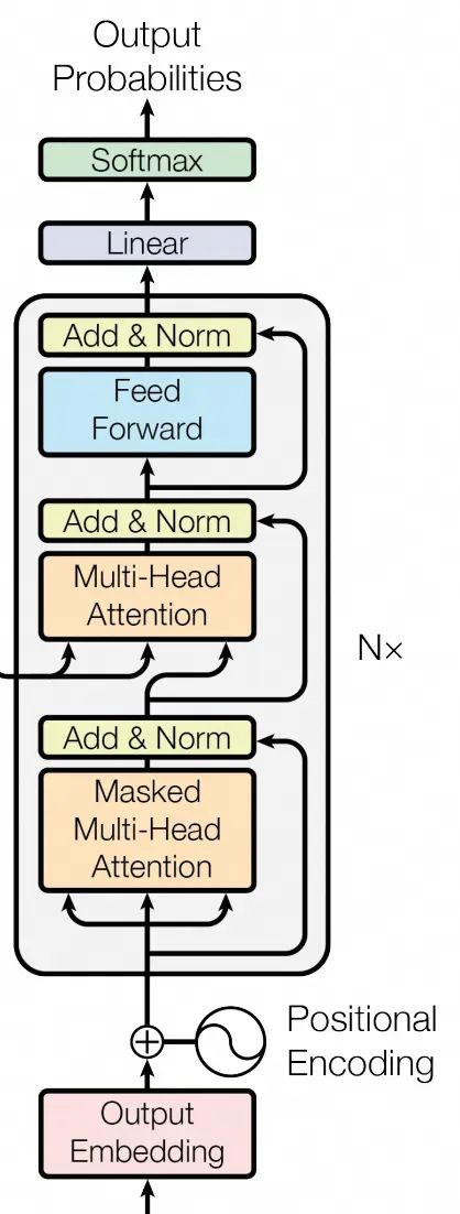
Implementing LLM from Bigram Model with 200 Lines of Python Code

Encapsulated into a Block class, allowing us to sequentially connect multiple Blocks, which is the meaning of “Nx” in the diagram.

Sometimes when we say a Transformer structure has N layers, it refers to the number of Blocks here.

+n_layer = 3# Number of blocks
+class Block(nn.Module):
+    def __init__(self, n_embed, n_head):
+        super().__init__()
+        head_size = n_embed // n_head
+        self.sa = MultiHeadAttention(n_head, head_size)
+        self.ffwd = FeedFoward(n_embed)
+
+    def forward(self, x):
+        x = self.sa(x)
+        x = self.ffwd(x)
+        return x

4. Residual Neural Network (Residual Connection)

The code can be found in babygpt_v7_residual_connection.py

This is a very simple structure that directly passes the input x across layers to subsequent layers, solving the gradient vanishing problem during training. The code is very straightforward (the more impressive the terminology in neural networks, the less code it corresponds to 😅, you read that right, just these two lines).

     def forward(self, x):
-        x = self.sa(x)
-        x = self.ffwd(x)
+        x = x + self.sa(x) # Used residual connection to retain original x information, avoiding gradient vanishing
+        x = x + self.ffwd(x)
         return x

5. Projection

The code can be found in babygpt_v8_projection.py

Projection is an operation that maps input data from the current vector space to another vector space. In our implementation, it is simply a linear layer. Its purpose is also to enhance the model’s expressive capability.

@@ -54,8 +54,9 @@ class FeedFoward(nn.Module):
         super().__init__()
         self.net = nn.Sequential(
-            nn.Linear(n_embed, n_embed),
+            nn.Linear(n_embed, n_embed * 4),
             nn.ReLU(), # Activation function that turns negative values to 0, keeps positive values unchanged
+            nn.Linear(n_embed * 4, n_embed),
         )
     def forward(self, x):
         return self.net(x)
@@ -64,9 +65,11 @@ class MultiHeadAttention(nn.Module):
     def __init__(self, num_heads, head_size):
         super().__init__()
         self.heads = nn.ModuleList([Head(head_size) for _ in range(num_heads)])
+        self.proj = nn.Linear(n_embed, n_embed) # Projection layer, mapping the multi-head attention output back to n_embed dimensional space
     def forward(self, x):
-        return torch.cat([h(x) for h in self.heads], dim=-1)
+        out = torch.cat([h(x) for h in self.heads], dim=-1)
+        return self.proj(out)

As shown in the code above, we added linear layers in two places. For the entire model, there is no difference other than increasing the parameters.

6. Layer Normalization (LayerNorm)

The code can be found in babygpt_v9_layer_norm.py

In neural networks, Layer Normalization is an important technique used to accelerate training and improve model stability. LayerNorm normalizes all features of a single sample to have a mean of 0 and a variance of 1, and then adjusts the distribution through learnable parameters.

As shown below:

>>> ln = torch.nn.LayerNorm(3)
>>> x = torch.tensor.randint(0, 10, (2,3)).float()
tensor([[9., 2., 4.],
        [5., 6., 9.]])
>>> ln(x)
tensor([[ 1.3587, -1.0190, -0.3397],
        [-0.9806, -0.3922,  1.3728]], grad_fn=<NativeLayerNormBackward0>)

The implementation is also very simple, using torch.nn.LayerNorm at some output locations for normalization, and I will not post the code here.

Note that the original Transformer paper uses Post-LayerNorm, where the output of each sub-layer (self-attention/feedforward network) undergoes LayerNorm after the residual connection, while the GPT series uses Pre-LayerNorm, which applies LayerNorm to the input before entering the sub-layer calculations, and then applies the residual connection. This structure makes training more stable and has become a standard for subsequent models (such as GPT-2/3, LLAMA, etc.).

7. Dropout

The code can be found in babygpt_v10_dropout.py

In machine learning, Dropout is a widely used regularization technique aimed at preventing neural networks from overfitting. It randomly drops the results of some neurons to force the model to learn more robust feature representations, as follows:

>>> x = torch.randint(0, 10, (2,3)).float()
>>> dp = torch.nn.Dropout(0.5)
>>> xtensor([[5., 9., 7.],
        [8., 3., 1.]])
>>> dp(x)
tensor([[10.,  0.,  0.],
        [ 0.,  6.,  0.]])

When the dropout rate is 0.5, executing dropout will randomly drop 50% of the input features.

Specifically, we added dropout to the outputs of Head, Multi-Head, and FeedForward.

Adjusting Parameters, Start Training

So far, we have implemented the complete “GPT-like” Transformer structure code. Let’s adjust the hyperparameters at the top of the code file.

The final complete code can be found in babygpt_v11_hyper_params.py[2], after deleting some comments, the code is exactly 200 lines long 😄 (in fact, there is a lot of code that can be simplified, but it is kept for simplicity).

-batch_size = 32 # Batch size
-block_size = 8 # Maximum length of each sequence
-learning_rate = 1e-2 # Learning rate
-n_embed = 32 # Dimension of the embedding layer
-n_head = 4 # Number of heads in multi-head attention
-n_layer = 3# Number of blocks
+batch_size = 64 # Batch size
+block_size = 256 # Maximum length of each sequence
+learning_rate = 3e-4 # Learning rate
+n_embed = 384 # Dimension of the embedding layer
+n_head = 6 # Number of heads in multi-head attention
+n_layer = 6# Number of blocks

Before adjustment, it was a “K-level super small model” with 3 layers, 4 heads, and 437,764 parameters.

After adjustment, it is a “15M model” with 6 layers, 6 heads, and 15,466,756 parameters, which can at least be measured in B units, being a “0.0155B” model.😄

The training and inference effects can be seen in the “final effect” at the beginning of the article.

Review and Next Steps

We have implemented a complete GPT-like Transformer architecture with 200 lines of code.

This model currently has 0.0155B parameters, compared to the smallest 0.5B of qwen2.5, it is still quite compact.

We have witnessed attention, QKV, and answered questions about what attention is and why there is kvcache.

Most people use AI through chat, and this current model still has a long way to go to achieve “conversational ability”. In the future, we will continue to complete the following:

Use a real tokenizer. Currently, a character-level correspondence table is used;
Use more data for pretraining and dialogue data for SFT, which should enable conversation;
Use more data for reinforcement learning to enhance inference capabilities;
Use Grouped Query Attention (GQA) to replace the current Multi-head Attention mechanism;
Introduce MoE architecture to increase experts;
……

Happy Hacking🏴☠️

References:

Improving Language Understanding by Generative Pre-Training: https://cdn.openai.com/research-covers/language-unsupervised/language_understanding_paper.pdf
Attention Is All Your Need: https://arxiv.org/abs/1706.03762
karpathy/nanoGPT: https://github.com/karpathy/nanoGPT Highly recommended, 99% of this series is directly copied from the work of the great Ak.

[1]https://github.com/simpx/buildyourownllm/blob/main/babygpt_v2_position.py

[2]https://github.com/simpx/buildyourownllm/blob/main/babygpt_v11_hyper_params.py

Multimodal Data Information Extraction

With the rapid development of information technology, data acquisition and processing have become particularly important. This solution provides multimodal file information extraction capabilities, utilizing advanced artificial intelligence technology to identify and parse various file formats, including text, images, audio, and video, thereby extracting valuable information and significantly enhancing data processing efficiency.

Click to read the original text for details.

Step 1: Initialize Input

Step 2: Calculate Key/Query/Value

Step 3: Calculate Attention Scores (Q·Kᵀ) and Scale

Step 4: Apply Mask

Step 5: Softmax Normalization

Step 6: Aggregate Value

Summary & kvcache

Related posts

Leave a Comment Cancel reply