 Click the top to follow for more content. Feel free to share. For details, contact Teacher Wang: 13521993969
Fitting of measurement data has wide applications in scientific research and engineering. Below are several commonly used fitting methods and how to implement them in the MATLAB environment.
In MATLAB, there are commands for fitting such as polyfit, lsqcurvefit, nlinfit, and the curve fitting tool cftool, which are sufficient to solve general engineering fitting problems. Below are several commonly used functions.
1
Polynomial Fitting
p=polyfit(x,y,n) performs polynomial fitting of the data, obtaining polynomial coefficients p arranged in descending order. The parameters x, y are vectors composed of data (xi,yi)(i=1,2,⋯,n), and n is the degree of the polynomial. For example:
x=[1, 3, 4, 6, 7];
y = [-2.1,-0.9,-0.6, 0.6, 0.9] ;
p = polyfit(x,y,1)
p =
0.5053 -2.5421
Thus, the fitting equation is:

Polynomial fitting can be reduced to a linear fitting problem. However, most nonlinear fitting problems cannot be transformed into linear fitting problems and require the direct use of nonlinear least squares algorithms. Below are several.
2
lsqnonlin() Function
The lsqnonlin() function is used to solve nonlinear least squares problems.
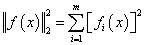
The format is as follows:
[x, resnorm, residual, exitflag, output, lambda, jacobian] = lsqnonlin(fun,x0,lb,ub,options)
where fun is the vector function; x0 is the initial point; lb, ub are the lower and upper bounds of the variables, respectively; options are the parameter choices set by the optimset function. The variable ~x is the local minimum of the nonlinear least squares problem; resnorm is the sum of squared residuals at x; residual is the residual value at x; exitflag is the exit condition; output is the output solving information; lambda are the Lagrange multipliers for the lower and upper bounds; Jacobian is the Jacobian matrix at x.
For example, to solve a nonlinear system of equations:
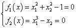
Set the initial point:
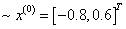
>> equs = @(x)[x(1)^2+x(2)^2-1; x(1)^3-x(2)]; x0 = [-0.8;0.6];
[x, resnorm, residual, exitflag, output, lambda, jacobian] = lsqnonlin(equs,x0)
Local minimum found.
Optimization completed because the size of the gradient is less than
the default value of the function tolerance.
<stopping criteria details>
x =
-0.8260
-0.5636
resnorm =
5.7708e-27
residual =
1.0e-13 *
0.3397
-0.6795
exitflag =
1
output =
firstorderopt: 1.9521e-13
iterations: 9
funcCount: 30
cgiterations: 0
algorithm: ‘trust-region-reflective’
stepsize: 1.7483e-07
message: ‘Local minimum found.…’
lambda =
lower: [2×1 double]
upper: [2×1 double]
jacobian =
(1,1) -1.6521
(2,1) 2.0470
(1,2) -1.1272
(2,2) -1.0000
3
lsqcurvefit() Function
The lsqcurvefit() is a nonlinear least squares fitting function, and its format is:
[x, resnorm, residual, exitflag, output, lambda, jacobian] = lsqcurvefit(fun,x0,xdata,ydata,lb,ub,options)
where fun is the vector function; x0 is the initial point; xdata, ydata are the fitting points; lb, ub are the lower and upper bounds of the variables, respectively; options are the parameter choices set by the optimset function. The variable x is the local minimum of the nonlinear least squares problem; resnorm is the sum of squared residuals at x; residual is the residual value at x; exitflag is the exit condition; output is the output solving information; lambda are the Lagrange multipliers for the lower and upper bounds; Jacobian is the Jacobian matrix at ~x.
For example, given data:
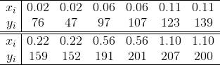
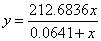
that satisfies the Michaelis-Menten equation:

Find parameters p1, p2.
xdata = [0.02, 0.02,0.06,0.06,0.11 ,0.11,0.22,0.22,0.56,0.56,1.10,1.10 ];
ydata = [76, 47,97,107,123,139,159,152,191,201,207,200];
fun = @(p,xdata)(p(1)*xdata./(p(2)+xdata)); x0 = [200;0.1];
p = lsqcurvefit(fun,x0,xdata,ydata)
After running, you can obtain:
p =
212.6836
0.0641
Thus, the fitting function is:
4
nlinfit() Function
The nlinfit() is a nonlinear regression function, and its format is:
[beta,r,J,Sigma,mse] = nlinfit(X,y,fun,beta0)
where X is the design matrix; y is the response variable; fun is the regression (fitting) function; beta0 is the initial parameters; beta is the optimal regression parameters; r is the residual; J is the Jacobian matrix; Sigma is the parameter covariance matrix; mse is the mean squared error.
For example, given data:
that satisfies the Michaelis-Menten equation:

Find parameters p1, p2.
x = [0.02, 0.02,0.06,0.06,0.11 ,0.11,0.22,0.22,0.56,0.56,1.10,1.10 ];
y = [76, 47,97,107,123,139,159,152,191,201,207,200];
fun = @(beta,x)(beta(1)*x./(beta(2)+x)); beta0 = [200;0.1];
beta = nlinfit(x,y,fun,beta0)
beta =
212.6836
0.0641
Thus, the fitting function is:
Source: This article is from Wang Fuchang’s Science Blog,Author:Wang Fuchang

Course Details Preview
1、Thermal-Fluid-Solid Coupling Theory and Numerical Simulation (Thermal-Structural Coupling, Conjugate Heat Transfer, Fluid-Solid Coupling, Thermal-Fluid-Solid Coupling)
2、Ls-Dyna Display Dynamics (Upper – Impact, Penetration, Explosion, Crack Propagation, Restart) (Lower – Thermal Coupling, Explicit-Implicit Coupling, Electromagnetic Coupling, Discrete Elements, Explicit Optimization)
4、Bolt Structure Steel Strength Check, Bolt Creep Simulation, Fatigue Life Prediction, and Bolt Fracture Analysis
5、ICEM Mesh Generation Technology (Mesh Size Control, Mesh Quality Control, Geometry Cleaning, Unstructured Mesh Generation, Block Hexahedral Mesh Generation)
6、Pro/E 3D Assembly and Motion Interference Simulation
7、nCode DesignLife Fatigue Prediction Typical Engineering Applications
8、Structural Topology, Parameter Optimization Design, and Engineering Reliability Analysis
Registration Method: Click the QR code below to enter the registration area

Zhengtai CAE, as a domestic expert in CAE application solutions, provides enterprises with fast, accurate, and comprehensive CAE application solutions, covering CAE software secondary development, CAE technology implementation and application, CAE technology consulting and training, involving aerospace, aviation, shipping, weapons, nuclear power, electrical science, automotive, machinery, electrical, and more. Over the past ten years, we have successfully provided customized CAE simulation solutions for more than 1,000 enterprises. Choose Zhengtai Science and Technology to bring unlimited possibilities to your enterprise.
Q: What other knowledge do you think needs attention?
Feel free to leave a message and share your thoughts with everyone. Please follow our WeChat public account.
For details, please contact 13521993969 Teacher Wang