Introduction to SVM

Face recognition is a frequently discussed topic in computer science and has gained significant attention due to the exponential growth of computing power. Face recognition has widespread applications in various fields such as robotics, biosecurity, and the automotive industry, involving the application of mathematical algorithms to input images to extract different features, indicating whether a face is present in the provided image. The Histogram of Oriented Gradients (HOG) is a traditional algorithm used to extract image features, such as pixel directions, and can be used with a Linear Support Vector Machine (SVM) to identify whether the input image is a face or not.

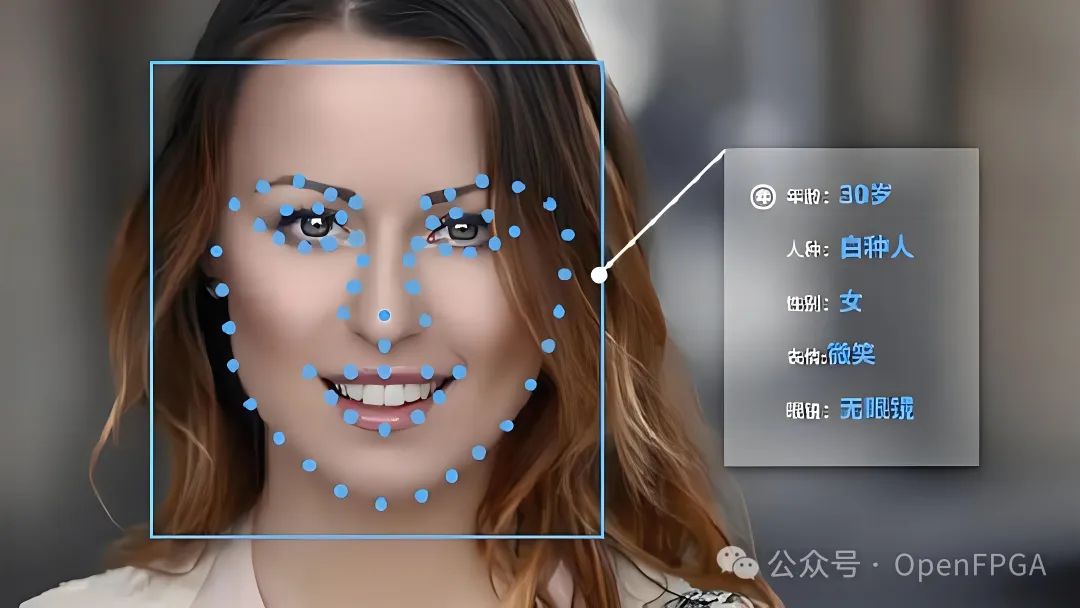
We will use the image below as a reference and test:

Image Processing

Convolution

The convolution of two functions is an important mathematical operation widely used in signal processing. In computer graphics and image processing, we typically use discrete functions (such as images) and apply a discrete form of convolution to eliminate high-frequency noise, sharpen details, or detect edges.

Convolution is a mathematical operation on two signals f and g, defined as:

In the image domain, we can think of convolution as the relationship between a single pixel and its neighboring pixels. This relationship is primarily applied to detect unique features such as color changes, brightness differences, and pixel periodicity.

The following diagram illustrates the convolution filter using a small 3 x 3 kernel. The filter is defined as a matrix where the center element weights the center pixel, and the other elements define the weights of the neighboring pixels. We can also say that the radius of a 3×3 kernel is 1, as only the “one-ring” neighborhood is considered during the convolution process. The behavior of convolution at the image boundary needs to be defined, where the kernel maps to undefined values outside the image.

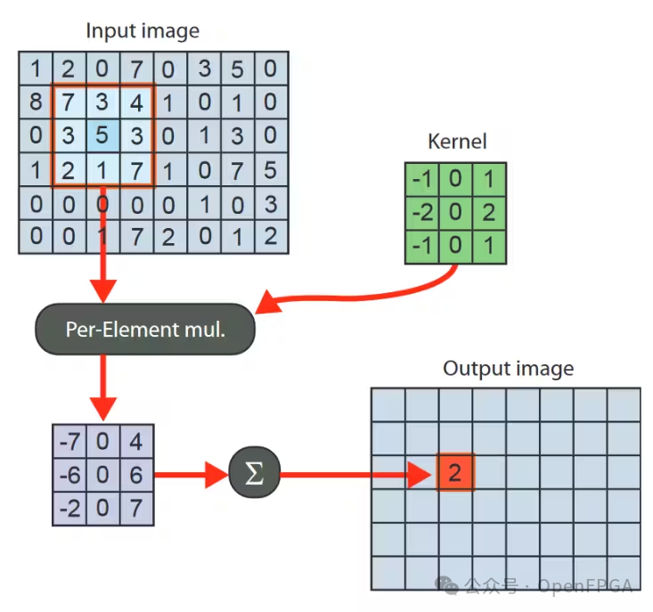
The convolution operation using a 3 x 3 window and a 3 x 3 kernel can be defined as follows:

static int convolve(unsigned int window[3][3], int kernel[3][3])
{
    int result = 0;

    for (int i = 0; i < 3; i++) {
        for (int j = 0; j < 3; j++) {
            result+= window[i][j] * kernel[i][j];
        }
    }

    return result;
}

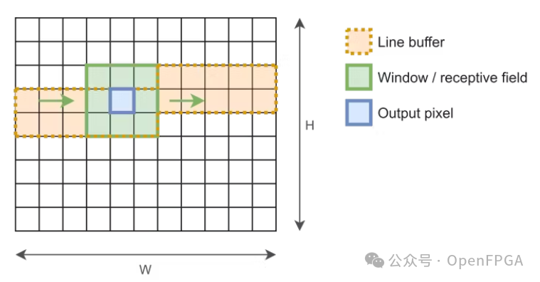
To perform convolution on the entire image, a sliding window technique can be applied. Starting from the first pixel, every 8 neighboring pixels are grouped into a square window, and the input pixels within the window are convolved with the kernel, producing a pixel value that is placed in the output image. This step is repeated until the end of the image.

Sobel

Edge detection is the most common method for detecting discontinuities in grayscale images. An edge is defined as a set of connected pixels located on a specific boundary between two regions.

If the input image is a color image, it should be converted to a grayscale image before applying the convolution operation.

Assuming each pixel is represented by a 32-bit unsigned integer, the code for converting RGB to grayscale is as follows:

#define R(pixel)    (((pixel) >> 16) & 0xFF)
#define G(pixel)    (((pixel) >> 8)  & 0xFF)
#define B(pixel)    (((pixel)      ) & 0xFF)

float rgb2gray(unsigned int pixel)
{
    return (R(pixel) * 0.2989 + G(pixel) * 0.5870 + B(pixel) * 0.1440);
}

After running, the test image will look like this:

The Sobel operator is one of the most commonly used operators in edge detection. The Sobel operator uses two 3×3 kernels convolved with the original image to compute approximations of the derivatives – one for horizontal changes and the other for vertical changes. If we define A as the source image, G x and G y are two images that contain the approximations of horizontal and vertical derivatives at each point, respectively, the calculations are as follows:

Using the previous convolution function, we can calculate the output image with the following code:

int dx = convolve(window, kernel_x);
int dy = convolve(window, kernel_y);

Where the window is defined as a 3 x 3 sliding window, and the kernels are the Sobel operator kernels used:

static int kernel_x[3][3] = {
    { 1,  2,  1},
    { 0,  0,  0},
    {-1, -2, -1}
};

static int kernel_y[3][3] = {
    { 1,  0, -1},
    { 2,  0, -2},
    { 1,  0, -1}
};

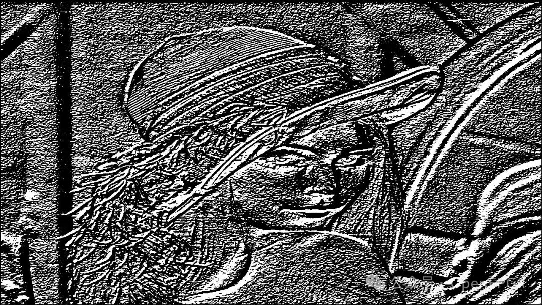
The image obtained after the convolution calculation is as follows:

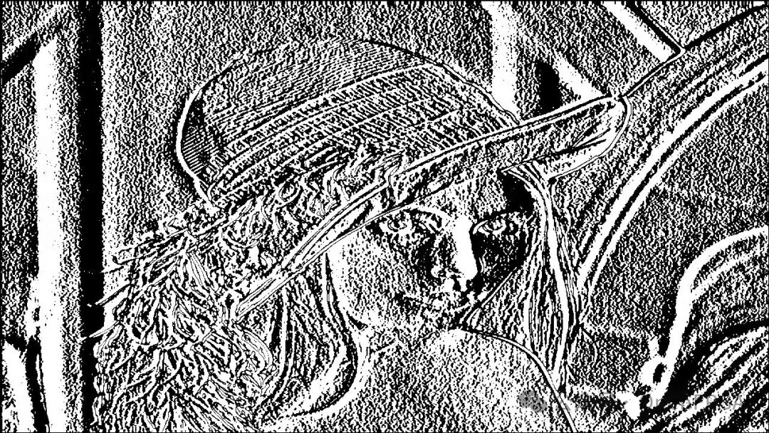
As seen, the vertical and horizontal details are enhanced and easier to observe. Although it helps, we need a more unique feature image that represents only the edges.

The next step is to combine these two images and obtain a bi-directional change image. We can do this by calculating the magnitude or intensity of each pixel value and the direction or angle that links the current pixel to another pixel in the edge line.

At each point in the image, the following method can be used to combine the resulting approximations to give the magnitude:

And the angle used:

The squareroot and atan2 functions have been implemented in the HLS namespace:

unsigned int magnitude = hls::sqrt(dx*dx + dy*dy);
int angle = hls::atan2(dx,dy);

The result is:

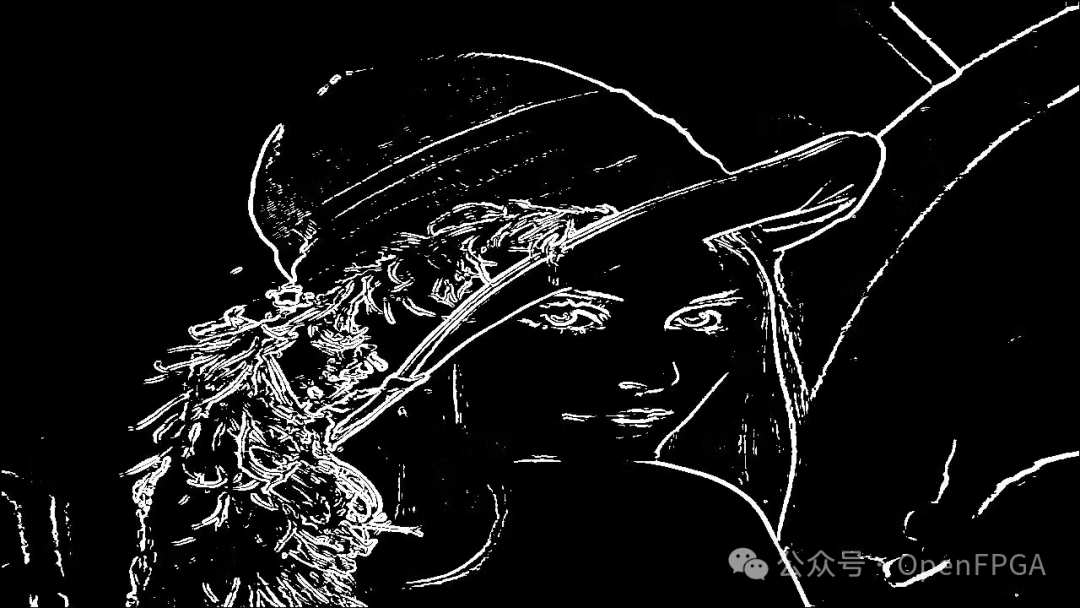
We have obtained a more focused image of edges. Nevertheless, edges can become wider in various forms. We need to use a technique called non-maximum suppression to suppress these false edges:

unsigned int nms(unsigned int mag[3][3], int ang) {
    unsigned int q,r;
    
    q = r = 255;
    
    if ((0 <= ang < 23) || (158 < ang <= 180)) {
        q = mag[1][2];
        r = mag[1][0];
    } else if (223 <= ang < 68) {
        q = mag[2][0];
        r = mag[0][2];
    } else if ( 68 <= ang < 113) {
        q = mag[0][1];
        r = mag[2][1];
    } else if ( 113 <= ang < 158) {
        q = mag[0][0];
        r = mag[2][2];
    }

    if (mag[1][1] >= q && mag[1][1] >= r)
        return mag[1][1];

    return 0;
}

Now the edges are thinner and more concise.

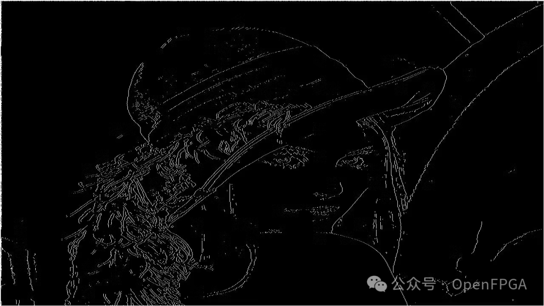
Implementation

As mentioned earlier, the input image is fed pixel by pixel in the form of a data stream. To apply the convolution operation, we need to package the data under a 3 x 3 window. This can be implemented using an architecture with two buffers, where the number of elements equals the width, if our input image:

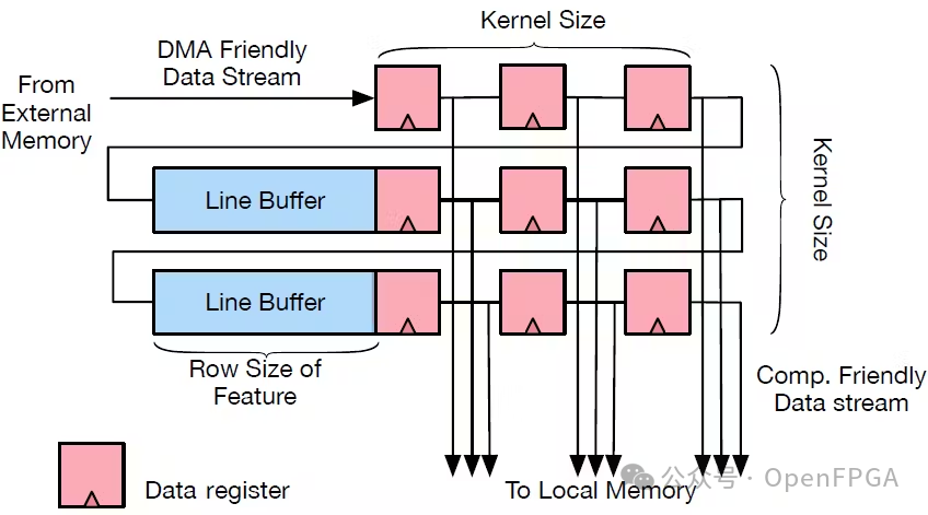
Here, there will be two auxiliary functions for moving the line buffer and the sliding window:

static void shift_w(unsigned int window[3][3], unsigned int v1, unsigned int v2,
                    unsigned int v3)
{
    window[0][0] = window[0][1];
    window[0][1] = window[0][2];
    window[0][2] = v1;
    window[1][0] = window[1][1];
    window[1][1] = window[1][2];
    window[1][2] = v2;
    window[2][0] = window[2][1];
    window[2][1] = window[2][2];
    window[2][2] = v3;
}

static void shift_b(unsigned int line_buffer[2][1280], int pos,
                    unsigned int val)
{
    line_buffer[0][pos] = line_buffer[1][pos];
    line_buffer[1][pos] = val;
}

Finally, we can package the entire process into an HLS function (see attached code).

After obtaining the code, it should also be tested. GIMP (https://www.oschina.net/p/gimp?hmsr=aladdin1e1) has a very cool feature that allows you to export images directly as header files. Assuming we export the test image to a file named image.h, we can utilize the following code to implement the functionality we want to test (see code at the end).

Another way to validate the HLS IP is to verify it directly on the FPGA.

The first step is to create a block design and add the synthesized Sobel IP to the repository:

Add the implemented IP, where one DMA provides data to it, and the other reads the output:

After generating the bitstream, we can validate the functionality.

The generated image should be similar to the simulated image.

Now we need to implement an architecture that directly inputs from the camera.

The first component is the Zynq processing system and the i2c controller for configuring the camera interface:

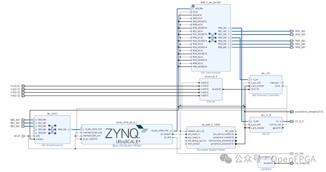
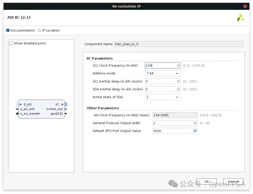
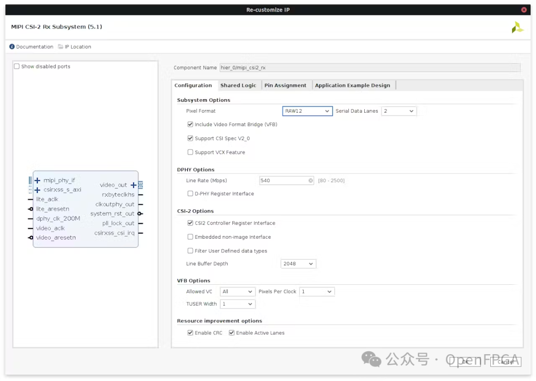
In terms of image flow, a MIPI controller and a Demosaic IP are needed to convert the stream to RGB24:

Finally, we add our image processing IP and VDMA:

HOG

Follow-up articles will introduce this separately, stay tuned~

SVM – Support Vector Machine

In machine learning, Support Vector Machines (SVM, also known as Support Vector Networks) are supervised learning models with associated learning algorithms used for analyzing data for classification and regression analysis. Given a set of training samples, each labeled as belonging to one of two categories, the SVM training algorithm builds a model that assigns new samples to one category or another, making it a non-probabilistic binary linear classifier (though methods like Platt scaling can be used to apply SVM in a probabilistic classification setting). The SVM model represents examples as points in space, mapping them to create a clear gap as wide as possible between different categories of examples. New examples are then mapped to the same space and predicted to belong to a certain category based on which side of the gap they fall on.

Code

https://github.com/cuciureansergiu/kv260_svm