X-Y display, also known as a scatter plot or cross-plot, provides a method for plotting one trace against another. This type of display can be used to compare two waveforms and show the relationship between them. A third parameter, such as frequency of occurrence, can be added to the two-dimensional plot as a variation in color or intensity.
Many classic and modern applications of the X-Y display mode can be found, ranging from the classic Lissajous figures used to measure phase or frequency ratios to state transition diagrams in modern digital communication systems. The X-Y plot can show whether a relationship exists between two variables. If a relationship exists, it can also indicate whether the relationship is linear or nonlinear and the direction of the relationship. This article will introduce some of these applications.
Lissajous Figures
A classic application of X-Y display is the Lissajous figure, which is created by plotting two sine waves against each other. For sine waves of the same frequency, this plot is used to measure the phase difference between the sine waves. With modern oscilloscopes, it is easier to obtain the phase difference between two signals using a single measurement parameter reading. If the sine waves have different frequencies, the frequency ratio can also be determined, as shown in Figure 1.
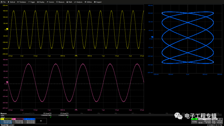
Figure 1: X-Y plot of two harmonically related sine waves, where the ratio of horizontal peaks to vertical peaks indicates an input signal frequency ratio of 2 to 5.
This plot shows that the relationship between the frequencies of the two input signals is 2 to 5. The actual measured frequencies are 1 MHz and 2.5 MHz, respectively.
Curve Tracer
With the help of an oscilloscope and an arbitrary waveform generator (AWG), X-Y plots can be used to characterize the V-I characteristics of semiconductor devices. Figure 2 shows the measurement results for a silicon diode.
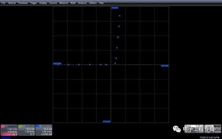
Figure 2: V-I curve formed by 12 voltage values generated by the AWG and the current flowing through the silicon diode.
The 12 pulse signals generated by the AWG increase the voltage amplitude from -5V to +5V. The oscilloscope’s sequence mode is used to acquire the voltage across the diode and the current through the diode, one pulse per sequence segment. The measured voltage and current parameters are summarized in a trend plot, with each point having a parameter value. The voltage is applied to the horizontal input axis of the X-Y display, scaled at 1 volt per division, while the current is applied to the vertical axis, with each division equal to 12.4 mA. The resulting X-Y plot displays the V-I characteristics of the diode. This quick testing is useful for things like matching components.
Orthogonal Signal Measurement
The orthogonal signal generation function uses two signals that are 90° out of phase to generate a phase-variable signal. The two signals added orthogonally define a vector with amplitude and phase. The X-Y plot supported by the X-Y cursor allows for viewing and measuring the vector phase and amplitude generated by the orthogonal input signals, as shown in Figure 3.
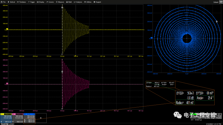
Figure 3: X-Y plot of two orthogonal signals showing the phase trace of the vector (the square sum of the signals). The X-Y cursor can read the vector amplitude (radius) and phase (angle) as well as Cartesian coordinate values.
The X-Y display allows visualization of the rotational vector tracking path defined by the square sum of two exponentially weighted RF pulses. The X-Y cursor reads the vector amplitude (radius) and phase relative to the X-axis, as well as the voltage of the source sampling points in channels 1 and 2. These cursor readings will track the X-Y, X-T, and Y-T waveforms. This means that any cursor measurement of the vector’s source components is being measured simultaneously. The X component of a 401 mV vector amplitude is 349.6 mV, while the Y component is 196.9 mV. This information is very useful in applications using orthogonal signals, such as radar and digital communications, as it can easily trace back to the sources of error for these vector parameters.
The X-Y display can also provide persistence display, allowing multiple traces that have been overwritten in the plot to remain visible. The persistence display function uses intensity or color to show the frequency of occurrence of the pixels displayed. Figure 4 shows an X-Y state transition diagram of a 16QAM signal with its in-phase (I) and quadrature (Q) components, where the I component is displayed based on the Q component. This X-Y display uses monochrome persistence.
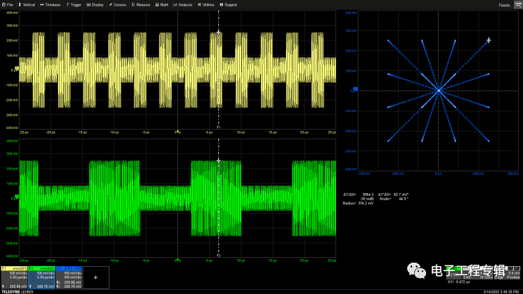
Figure 4: X-Y plot presented in monochrome persistence. In this diagram, the data states of the state transition diagram are shown as bright points, while the multiple transitional phase paths are shown brighter.
The state transition diagram shows the data states at the end of each transition path and marks the paths between data states. The time spent by the waveform at each data state is greater than the time spent on the transition paths, so the data states appear as brighter points on the X-Y plot. The four phase states of 45°, 135°, 225°, and 315° are written twice with two different vector amplitudes, appearing brighter as well. Thus, the persistence plot provides additional information about this measurement, including a clearer display of overlapping vectors.
Power-Related X-Y Measurements
X-Y display can be used for measuring power switching devices. Figure 5 plots the relationship between voltage and current on a power FET to ensure the device operates within its safe operating area (SOA).
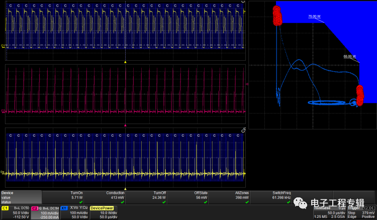
Figure 5: X-Y plot used to measure the operating area (SOA) of a power FET, showing the relationship between drain current and drain-source voltage. The “Pass/Fail” test compares the X-Y plot with a template, with red circles indicating failures.
The drain-source voltage (VDS) across the FET is applied to the horizontal axis, while the drain current is applied to the vertical axis. The vertical portion of the X-Y plot indicates that the FET is in the on state, where the current increases while VDS remains nearly constant. The horizontal loop displays the FET turning off, with zero current and oscillating voltage. The middle trace represents the switching transition process of the device when dissipating power. This test can verify whether the device exceeds its voltage, current, and power limits.
The blue area is the “Pass/Fail” template used to monitor measurement results. The X-Y trace should not intersect with the template. If it does, it indicates a test failure, marked as a failure with a red circle. Additionally, the “Pass/Fail” test has several response options, including hardware and software, to indicate the test status for response actions.
Another power-related X-Y measurement is the measurement of the magnetic properties of inductive devices. Figure 6 shows the measured hysteresis curve of an inductor.
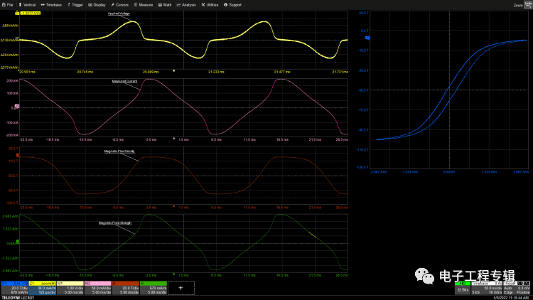
Figure 6: Hysteresis curve graph plotting magnetic flux density as a function of magnetic field strength.
The inputs for the hysteresis graph are magnetic field strength and magnetic flux density. Magnetic field strength is calculated from the current flowing through the inductor, while magnetic flux density is obtained by integrating the applied voltage. The oscilloscope used in this article has a software option for power measurements that can perform these calculations based on known coil geometries (cross-sectional area and magnetic circuit length), voltage, and current. The area within the hysteresis loop represents the energy loss per cycle, commonly referred to as hysteresis loss.
Mechanical Measurements
X-Y plots can also be used to analyze mechanical devices. This requires appropriate sensors to convert mechanical parameters into proportional electrical signals. The pressure-volume graph of an engine is a great example of a mechanical device X-Y plot, as shown in Figure 7.
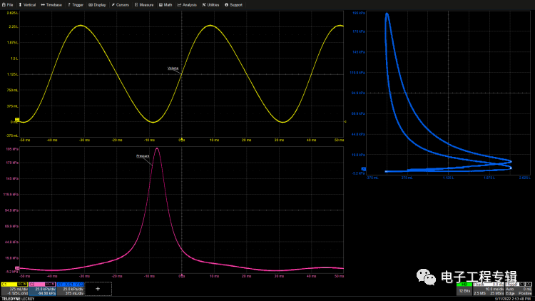
Figure 7: X-Y plot showing pressure as a function of the internal combustion engine cylinder volume.
The pressure values are read by a pressure sensor connected to the spark plug of the cylinder. The volume is calculated by a rotary encoder based on the measured crank angle. Both sensors utilize the oscilloscope’s rescaling feature, allowing measurements in standard pressure and volume units, in this case, pascals and liters. The PV diagram has two loops. The larger one above represents the power stroke, while the one below represents the exhaust stroke. The mechanical work produced by the engine during each cycle is proportional to the area within the PV diagram loop. The power stroke represents positive work, while the exhaust stroke represents negative work.
Conclusion
Clearly, the X-Y display is a very useful tool for interpreting measurement results. It can help designers compare signals, display the relationships between the plotted variables, and graphically show the vector amplitude and phase of orthogonal inputs. It can also provide information about energy contributions or losses during the cycle. This is a tool that engineers should keep in mind when learning about the dual-trace applications of digital oscilloscopes.