Abstract

Language models have been successfully used to model natural signals such as images, speech, and music. A key component of these models is high-quality neural compression models that can compress high-dimensional natural signals into lower-dimensional discrete tokens. To this end, we propose a high-fidelity universal neural audio compression algorithm that can compress 44.1 KHz audio into tokens at only 8 kbps bandwidth, achieving a compression ratio of 90 times. We achieved this by combining the latest advancements in high-fidelity audio generation with better vector quantization techniques from the image domain and improving adversarial and reconstruction losses. We use a single universal model to compress all types of audio (such as speech, environmental sounds, music, etc.), making it widely applicable for generative modeling of all audio. We compared our method with existing audio compression algorithms and found that our approach significantly outperforms them. We provide detailed ablation experiments for each design choice and offer open-source code and trained model weights. We hope our work lays the foundation for the next generation of high-fidelity audio modeling.

1. Introduction

Generating high-resolution audio is challenging due to its high dimensionality (approximately 44,100 audio samples per second) and the structure present at different time scales, which has both short-term and long-term dependencies. To address this issue, audio generation is typically divided into two stages: 1) predicting audio based on some intermediate representation (such as mel-spectrograms) [24, 28, 19, 30], and 2) predicting intermediate representations based on some conditional information (such as text) [35, 34]. This can be interpreted as a hierarchical generative model with observed intermediate variables. Naturally, another form is to use a variational autoencoder (VAE) framework to learn these intermediate variables, using learned conditional priors to predict latent variables given conditions. This form, which uses continuous latent variables and trains a powerful prior through regularized flows, has achieved considerable success in speech synthesis [17, 36]. A closely related idea is to train the same variational autoencoder using VQ-VAE [38], where discrete latent variables are adopted. It can be argued that discrete latent variables are a better choice because powerful autoregressive models can be used to train expressive priors, which have been developed to model distributions over discrete variables [27]. Specifically, transformer language models [39] have demonstrated the ability to scale in data and model capacity, learning complex distributions such as text [6], images [12, 44], audio [5, 41], and music [1]. While modeling priors is straightforward, modeling discrete latent codes using quantized autoencoders remains a challenge. Learning these discrete codes can be interpreted as a lossy compression task, where the audio signal is compressed into a discrete latent space by vector quantizing the representations of the autoencoder using a fixed-length codebook. This audio compression model needs to satisfy the following properties: 1) high-fidelity reconstruction of audio while avoiding artifacts. 2) achieving high compression rates and temporal scaling while learning a compact representation that discards low-level imperceptible details while retaining high-level structure [38, 33]. 3) using a single universal model to handle all types of audio, such as speech, music, environmental sounds, different audio codecs (such as mp3), and different sampling rates.

Despite recent neural audio compression algorithms like SoundStream [46] and EnCodec [8] partially meeting these properties, they often encounter the same issues faced by GAN-based generative models. Specifically, these models exhibit audio artifacts such as pitch artifacts [29], pitch and periodic artifacts [25], and fail to model high frequencies well, resulting in generated audio that is noticeably different from the original audio. These models are often fine-tuned for specific types of audio signals (such as speech or music), making it difficult to model general sounds. We make the following contributions:

• We propose an improved RVQGAN, a high-fidelity universal audio compression model that can compress 44.1 KHz audio into discrete codes at a bitrate of 8 kbps (approximately 90 times compression) while minimizing quality loss and reducing artifacts. Our method significantly outperforms existing state-of-the-art methods when evaluated at lower bitrates (higher compression) using quantitative metrics and qualitative listening tests.
• We identify a key issue with existing models, where codebook collapse (where parts of the code are unused) prevents these models from fully utilizing bandwidth, and address it with improved codebook learning techniques.
• We identify the side effect of quantizer dropout—this technique aims to allow a single model to support variable bitrates but actually reduces the quality of full-bandwidth audio, and propose solutions to mitigate this issue.
• We made impactful design changes to existing neural audio codecs, including adding periodic inductive bias, multi-scale STFT discriminators, multi-scale mel losses, and provide detailed ablation studies and intuitions to support these changes.
• Our proposed method is a universal audio compression model capable of handling speech, music, environmental sounds, different sampling rates, and audio encoding formats.

2 Related Work

High-fidelity neural audio synthesis: Recently, generative adversarial networks (GANs) have become a solution for generating high-quality audio and achieving fast inference speeds, thanks to feedforward (parallel) generators. MelGAN [19] successfully trained a GAN-based spectrogram inversion (neural vocoder) model. It introduced a multi-scale waveform discriminator (MSD) to penalize structures at different audio resolutions and used feature matching loss to minimize the L1 distance between the discriminator feature maps of real and synthesized audio. HifiGAN [18] optimized this scheme by introducing a multi-period waveform discriminator (MPD) for high-fidelity synthesis and adding auxiliary mel reconstruction loss to accelerate training. UnivNet [16] introduced a multi-resolution spectrogram discriminator (MRSD) to generate audio with clear spectrograms. BigVGAN [21] extended the HifiGAN scheme by introducing periodic inductive bias using the Snake activation function [47]. It also replaced the MSD in HifiGAN with MRSD, improving audio quality and reducing pitch and periodic artifacts [25]. Although these GAN-based learning techniques are used for vocoders, these schemes can also be easily applied to neural audio compression. Our improved RVQGAN model closely follows the training scheme of BigVGAN with some key modifications. Our model uses a new multi-band multi-scale STFT discriminator to alleviate aliasing artifacts and employs multi-scale mel reconstruction loss to better model fast transients.

Neural audio compression models: VQ-VAE [38] has been the mainstream approach for training neural audio codecs. The first VQ-VAE-based speech codec was proposed in [13], operating at a rate of 1.6 kbps. This model used the original architecture from [38], equipped with a convolutional encoder and an autoregressive WaveNet [27] decoder. SoundStream [46] is one of the first universal compression models that supports processing multiple audio types and compressing at different bitrates using a single model. It uses fully causal convolutional encoder and decoder networks and performs residual vector quantization (RVQ). The model is trained using the VQ-GAN [12] formulation, optimizing by adding adversarial loss, feature matching loss, and multi-scale spectral reconstruction loss. EnCodec [8] closely follows the SoundStream scheme and makes some modifications to improve quality. EnCodec uses multi-scale STFT discriminators and multi-scale spectral reconstruction loss. They use a loss balancer that adjusts loss weights based on the scale of gradients in the discriminator.

Our proposed method also uses a convolutional encoder-decoder architecture, residual vector quantization, and adversarial loss, and perceptual loss. However, our scheme has several key differences: 1) We introduce periodic inductive bias by using the Snake activation function [47, 21]. 2) We improve codebook learning by mapping encodings to a low-dimensional space [44]. 3) We achieve a stable training scheme by adopting best practices for adversarial and perceptual loss design, fixing loss weights, and not requiring a complex loss balancer. We find that these changes allow our model to use bandwidth effectively, approaching optimal usage. This enables our model to outperform EnCodec even at a bitrate that is three times lower.

Language modeling of natural signals: Neural language models have achieved great success in various tasks, demonstrating strong contextual learning capabilities in open-ended text generation [6]. A key component of these models is the self-attention mechanism [39], which can model complex long-term dependencies, but the computational cost grows quadratically with the sequence length. This cost is unacceptable for natural signals with very high dimensionality, such as images and audio, necessitating compressing the mapping to discrete representation space. This mapping is typically learned using VQ-GANs [12, 44], followed by training an autoregressive Transformer to handle discrete tokens. This approach has achieved success in fields such as images [45, 44, 32], audio [5, 41], video, and music [9, 1]. Codecs like SoundStream and EnCodec have been used to generate audio models, such as AudioLM [5], MusicLM [1], and VALL-E [41]. Our proposed model can serve as an alternative to the audio tokenization models used in these methods, providing higher audio fidelity and achieving more efficient learning due to the advantages of our maximum entropy code representation.

3 Improved RVQGAN Model

Our model builds upon the VQ-GANs framework, following the same pattern as SoundStream [46] and EnCodec [8]. Our model uses a fully convolutional encoder-decoder network from SoundStream, employing a selected stride factor for temporal downsampling. Following recent literature, we use residual vector quantization (RVQ) to quantize encodings, which is a method that recursively quantizes the residual after an initial quantization step, using different codebooks. During training, quantizer dropout is applied to allow a single model to operate at multiple target bitrates. Our model also uses frequency domain reconstruction loss and is trained in conjunction with adversarial loss and perceptual loss. An audio signal sampled at a rate of with an encoder stride factor of M and layers of RVQ generates a discrete code matrix of shape , where S is the frame rate defined as . Table 1 compares our proposed model with baseline models, comparing compression factors and the frame rates of latent codes. Note that the mentioned target bitrate is an upper limit, as all models support variable bitrates. Our model outperforms all baseline methods in terms of compression factor while also surpassing them in audio quality, as we will demonstrate later. Finally, lower frame rates are desirable when training language models based on discrete codes, as they produce shorter sequences.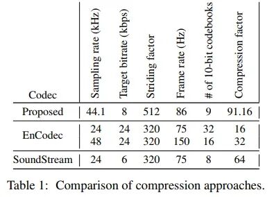

3.1 Periodic Activation Function

Audio waveforms often exhibit high periodicity (especially in voiced components, music, etc.). Although current non-autoregressive audio generation architectures can generate high-fidelity audio, they often exhibit abrupt pitch and periodic artifacts [25]. Additionally, common neural network activation functions (such as Leaky ReLU) perform poorly when inferring periodic signals and exhibit poor out-of-distribution generalization in audio synthesis [21]. To introduce periodic inductive bias into the generator, we adopted the Snake activation function proposed by Liu et al. [47] and introduced it into the audio domain in the BigVGAN neural speech coding model [21]. It is defined as: , where α controls the frequency of the signal’s periodic components. In our experiments, we found that replacing the Leaky ReLU activation function with the Snake function was a significant change that greatly improved audio fidelity (Table 2).

3.2 Improved Residual Vector Quantization

While vector quantization (VQ) is a common method for training discrete autoencoders, it faces many practical difficulties during training. Ordinary VQ-VAEs suffer from low codebook usage due to poor initialization, resulting in a large portion of the codebook being unused. This reduction in effective codebook size leads to a hidden decrease in target bitrate, which in turn affects reconstruction quality. To address this issue, recent audio codec methods have adopted k-means clustering to initialize codebook vectors and manually perform random restarts when certain codebooks are unused for several batches [9]. However, we found that the EnCodec model trained with the same codebook learning method (Proposed w/ EMA) at a target bitrate of 24 kbps, as well as our proposed model, still faced the issue of insufficient codebook utilization (Figure 1).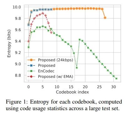

To solve this problem, we borrowed two key techniques introduced in the improved VQGAN image model [44] to enhance codebook utilization: factorized encoding and L2 normalized encoding. Factorization decouples code lookup and code embedding by performing code lookup in a low-dimensional space (8 or 32 dimensions) while retaining code embeddings in a high-dimensional space (1024 dimensions). Intuitively, this can be explained as using only the principal components of the input vector for code lookup, maximizing the variance explained by the data. Normalizing the encoding and codebook vectors with L2 transforms the Euclidean distance into cosine similarity, which helps with stability and quality [44]. These two techniques, along with the overall model formulation, significantly improved codebook utilization, thereby enhancing bitrate efficiency (Figure 1) and reconstruction quality (Table 2), while also being easier to implement. Our model can be trained using the original VQ-VAE codebook and commitment loss [38] without k-means initialization or random restarts. The equation for the modified codebook learning process is provided in Appendix A.

3.3 Quantizer Dropout Rate

The quantizer dropout rate was first introduced in SoundStream [46] for training a compression model with variable bitrates. The number of quantizers Nq determines the bitrate, so for each input example, we randomly select and only use the first n quantizers during training. However, we noticed that applying quantizer dropout at full bandwidth reduces audio reconstruction quality (Figure 2).

To address this issue, we instead apply quantizer dropout to each input example with a certain probability p. Interestingly, we found that a dropout probability p = 0.5 yields reconstruction quality very close to the baseline at lower bitrates while narrowing the gap with the full bandwidth quality of the model trained without quantizer dropout (p = 0.0).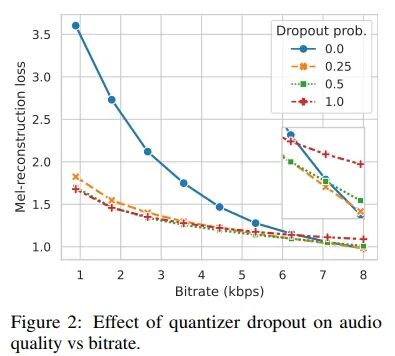

3.4 Discriminator Design

Similar to previous work, we use multi-scale (MSD) and multi-period waveform discriminators (MPD), which help improve audio fidelity. However, the spectrogram of generated audio may still appear blurry, especially in the high-frequency part, where excessive smoothing artifacts can occur [16]. To address these artifact issues, UnivNet proposed a multi-resolution spectrogram discriminator (MRSD), and BigVGAN [21] found that it also helps reduce pitch and periodic artifacts. However, using magnitude spectrograms loses phase information, which could be used by the discriminator to penalize phase modeling errors. Additionally, we found that high-frequency modeling remains a challenge for these models, especially at high sampling rates.

To address these issues, we employed a complex STFT discriminator [46] and processed it at multiple time scales [8], finding that this approach works better in practice and improves phase modeling capability. Furthermore, we found that splitting the STFT into sub-bands slightly improves high-frequency predictions and alleviates aliasing artifacts, as the discriminator can learn discriminative features for specific sub-bands and provide stronger gradient signals to the generator. Multi-band processing was previously proposed in [43] for predicting audio sub-bands, which are then summed to generate complete audio.

3.5 Loss Functions

Frequency Domain Reconstruction Loss: While it is known that mel reconstruction loss [18] can improve stability, fidelity, and convergence speed, multi-scale spectral loss [42, 11, 15] encourages modeling frequencies at multiple time scales. In our model, we combine these two approaches by using L1 loss on the mel spectrogram, which is computed using a window length of [32, 64, 128, 256, 512, 1024, 2048] and a hop length of window_length / 4. We specifically found that using a minimum hop size of 8 improves modeling of very fast transients, which is particularly common in music.

EnCodec [8] used a similar loss formulation but included both L1 and L2 loss terms, and the fixed bin size of the mel frequency spectrogram was 64. We found that fixing the bin size of the mel frequency spectrogram leads to gaps in the spectrogram at low filter lengths. Therefore, we used mel frequency spectrogram bin sizes of [5, 10, 20, 40, 80, 160, 320], which correspond to the above filter lengths and were confirmed to be correct through manual inspection.

Adversarial Loss: Our model uses a multi-period discriminator [18] for waveform discrimination while using the proposed multi-band multi-scale STFT discriminator for frequency domain discrimination. We use the HingeGAN [22] adversarial loss formulation and apply L1 feature matching loss [19].

Codebook Learning: We use the simple codebook and commitment loss from the original VQ-VAE formulation [38] and backpropagate gradients to the codebook lookup through a straight-through estimator [3].

Loss Weighting: We use a loss weight of 15.0 for multi-scale mel loss, 2.0 for feature matching loss, and weights of 1.0 and 0.25 for adversarial loss and codebook commitment loss, respectively. These weights are consistent with recent work [18, 21] (which used a weight of 45.0 for mel loss), but we performed simple scaling based on the multiple scales used and the log10-based mel loss calculation. We did not use the loss balancer proposed in EnCodec [8].

4 Experiments

4.1 Data Sources

We trained our model on a large dataset containing speech, music, and environmental sounds. For speech, we used the DAPS dataset [26], clear speech segments from the DNS Challenge 4 [10], the Common Voice dataset [2], and the VCTK dataset [40]. For music, we used the MUSDB dataset [31] and the Jamendo dataset [4]. Finally, for environmental sounds, we used balanced and unbalanced training segments from the AudioSet dataset [14]. All audio was resampled to 44 kHz.

During training, we extracted short segments from each audio file and normalized them to -24 dB LUFS. The only data augmentation method we applied was randomly and uniformly changing the phase of the segments. For evaluation, we used evaluation segments from the AudioSet dataset [14], two speakers (F10, M10) retained in the DAPS dataset [26] for speech testing, and the test set from the MUSDB dataset [31]. We extracted 3000 ten-second segments (1000 from each domain) as our test set.

4.2 Balanced Data Sampling

We paid particular attention to how we sampled from our dataset. Although our dataset has been resampled to 44 kHz, the data within it may be bandwidth-limited in some way. That is, some audio may have original sampling rates far below 44 kHz, especially in speech data, which is particularly common (e.g., Common Voice data is typically 8-16 kHz). When training the model at different sampling rates, we found that the resulting model often struggled to reconstruct content above a certain frequency. Upon investigation, we found that this threshold frequency corresponds to the average true sampling rate of our dataset.

To address this issue, we introduced a balanced data sampling technique. First, we divided the dataset into known full-band and data sources where we could not determine the maximum frequency. The known full-band data sources confirm the presence of energy reaching the target Nyquist frequency (22.05 kHz). When sampling batches, we ensured to sample a full-band item. Finally, we ensured that the number of items in each domain (speech, music, and environmental sounds) was equal in each batch. In our ablation studies, we will examine the impact of this balanced sampling technique on model performance.

4.3 Model and Training Recipe

Our model consists of a convolutional encoder, a residual vector quantizer, and a convolutional decoder. The basic building block of the network is a convolutional layer that can upsample or downsample the input audio waveform based on stride, followed by a residual layer composed of alternating convolutional layers and the nonlinear Snake activation function. Our encoder has 4 layers, each downsampling the input audio waveform at rates of [2, 4, 8, 8]. Our decoder has 4 corresponding layers, upsampling at rates of [8, 8, 4, 2]. We set the dimension of the decoder to 1536. Overall, our model has 76 million parameters, with 22 million in the encoder and 54 million in the decoder. We also experimented with decoders of 512 dimensions (31 million parameters) and 1024 dimensions (49 million parameters).

We used a multi-period discriminator [8] and a complex multi-scale STFT discriminator. For the former, we used periods of [2, 3, 5, 7, 11]; for the latter, we used window lengths of [2048, 1024, 512], with a stride set to one-fourth of the window length. For the STFT band splitting, we used bandwidth limits of [0.0, 0.1, 0.25, 0.5, 0.75, 1.0]. For reconstruction loss, we used the distance between the reconstructed waveform and the ground truth’s log mel spectrogram. The window lengths were set to [32, 64, 128, 256, 512, 1024, 2048], with corresponding mel counts of [5, 10, 20, 40, 80, 160, 320]. The stride length was one-fourth of the window length. We also used feature matching and codebook loss, as described in Section 3.5.

In our ablation studies, we set a batch size of 12 for each model and trained for 250k iterations. The actual training took about 30 hours using a single GPU. In our final model, we used a batch size of 72 and trained for 400k iterations. The audio segments we trained on were 0.38 seconds long. We used the AdamW optimizer [23], with a learning rate set to 1e-4, and , for the generator and discriminator. We decay the learning rate at each step, with a decay factor of .

4.4 Objective and Subjective Metrics

To evaluate our model, we used the following objective metrics:

1. ViSQOL: [Z] is an intrusive perceptual quality metric that estimates the mean opinion score by using spectral similarity to the ground truth.

2. Mel Distance: The distance between the reconstructed waveform and the ground truth waveform’s log mel spectrogram. The configuration of this loss is the same as described in Section 3.5.

3. STFT Distance: The distance between the reconstructed waveform and the ground truth waveform’s log magnitude spectrogram. We used window lengths of [2048, 512]. Compared to mel distance, this metric captures fidelity better in the high-frequency part.

4. Scale-Invariant Source-to-Distortion Ratio (SI-SDR) [20]: The distance between waveforms, similar to signal-to-noise ratio, but modified to be insensitive to scale differences. When considered alongside spectral metrics, SI-SDR can indicate the quality of audio phase reconstruction.

5. Bitrate Efficiency: We calculate bitrate efficiency by summing the entropy (in bits) of each codebook when applied to a large test set, then dividing by the total bits of all codebooks. For efficient bitrate utilization, the ideal bitrate efficiency should be close to 100%, while lower percentages indicate that the bitrate is not being fully utilized.

We also conducted a MUSHRA-like listening test, which included a hidden reference but no low-pass anchor. In the test, 10 expert listeners rated 12 randomly selected 10-second samples, drawn from our evaluation set, including 4 samples from each domain: speech, music, and environmental sounds. We compared our system’s performance at 2.67 kbps, 5.33 kbps, and 8 kbps with EnCodec’s performance at 3 kbps, 6 kbps, and 12 kbps.

4.5 Ablation Studies

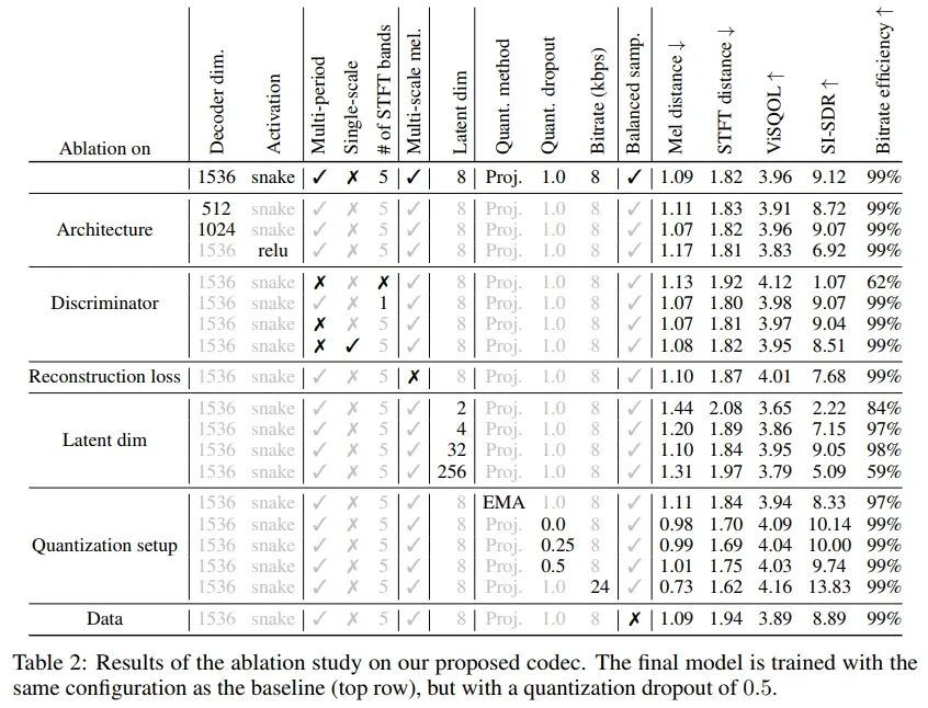
We conducted comprehensive ablation studies on our model, changing each component of the training recipe and model configuration one by one. To compare different models, we used the four objective metrics described in Section 4.4. Our ablation study results are shown in Table 2.

Architecture:

We found that changing the dimension of the decoder has a certain impact on performance, with smaller models generally performing worse across all metrics. However, the model with a decoder dimension of 1024 performed similarly to the baseline, indicating that smaller models can still be competitive. The most impactful change was replacing the ReLU activation function with the Snake activation function. This change significantly improved SI-SDR and other metrics. Similar to the results in BigVGAN [21], we found that the periodic inductive bias of the Snake activation function aids in waveform generation. For our final model, we used the maximum decoder dimension (1536) and the Snake activation function.

Discriminator:

Next, we removed or changed the discriminators one by one to observe their impact on the final results. First, we found that the multi-band STFT discriminator did not significantly improve other metrics except for SI-SDR. However, when examining the spectrogram of the generated waveforms, we found that the multi-band discriminator effectively alleviated high-frequency aliasing. The upsampling layers of the decoder introduce significant aliasing artifacts [29]. The multi-band discriminator can more easily detect these aliasing artifacts and feedback to the generator to remove them. Since the magnitude of aliasing artifacts is very small, their impact on our objective metrics is minimal. Therefore, we retained the multi-band discriminator.

We found that adversarial loss is crucial for the quality of output audio and bitrate efficiency. When trained with only reconstruction loss, bitrate efficiency dropped from 99% to 62%, while SI-SDR dropped from 9.12 to 1.07. Other metrics capturing spectral distance were less affected. However, this model’s audio exhibited many artifacts, including buzzing, as it failed to learn phase reconstruction. Finally, we found that replacing the multi-period discriminator with the single-scale waveform discriminator proposed in MelGAN [19] led to a deterioration in SI-SDR. We retained the multi-period discriminator.

Impact of Low Stride Reconstruction Loss:

We found that low-stride reconstruction is crucial for waveform loss and modeling fast transients and high frequencies. When replaced with single-scale high-stride mel reconstruction (80 mel, window length of 512), SI-SDR significantly decreased (from 9.12 to 7.68). Subjectively, we found that this model performed better at capturing certain types of sounds, such as cymbal crashes, buzzing, alarm sounds, and singing voices. We retained the multi-scale mel reconstruction loss in the final recipe.

Potential Dimension of Codebook:

The potential dimension of the codebook has a significant impact on bitrate efficiency and reconstruction quality. If set too low or too high (e.g., 2 or 256), quantitative metrics significantly deteriorate, and bitrate efficiency drops sharply. Lower bitrate efficiency effectively reduces bandwidth, which can impair the generator’s modeling capability. As the generator’s performance declines, the discriminator often “wins,” leading the generator to fail to learn to produce high-quality audio. We found that 8 is the optimal value for the potential dimension.

Quantization Settings:

We found that using exponential moving average as the codebook learning method (as done in EnCodec [8]) led to poorer metrics, especially in SI-SDR. It also resulted in lower codebook utilization across all codebooks (Figure 1). Considering its increased implementation complexity (requiring K-Means initialization and random restarts), we retained the simpler projection lookup method for learning the codebook and used commitment loss. Next, we noted that the quantizer dropout rate significantly impacts quantitative metrics. However, as shown in Figure 2, a dropout rate of 0.0 resulted in poor reconstruction and less codebook usage. Since this made downstream generative modeling tasks challenging, we ultimately used a dropout rate of 0.5 in our final model. This achieved a good balance between full bitrate and lower bitrate. Finally, we demonstrated that increasing the maximum bitrate of our model from 8 kbps to 24 kbps could achieve excellent audio quality, surpassing all other model configurations. However, for our final model, we chose to train at lower bitrates to maximize compression.

Balanced Data Sampling:

When removing balanced data sampling, metrics generally deteriorated. Empirically, we found that without balanced data sampling, the maximum frequency of the waveforms generated by the model was approximately 18 kHz. This aligns with the maximum frequency preserved by various audio compression algorithms (such as MPEG), which constitute the majority of our dataset. By employing balanced data sampling, we could sample as much as possible from high-quality datasets (e.g., DAPS) and bandwidth-limited audio from unknown quality datasets (e.g., Common Voice). This resolved the issue, allowing our codec to reconstruct both full-band audio and bandwidth-limited audio.

4.6 Comparison with Other Methods

We now compare the performance of our final model with competitive benchmarks: EnCodec [8], Lyra [46], and Opus [37], which is a popular open-source audio codec. For EnCodec, Lyra, and Opus, we used the publicly available open-source implementations provided by the authors. We compared using objective and subjective evaluations at different bitrates. The results are shown in Table 3. We found that the proposed codec outperformed all competing codecs in both objective and subjective metrics at all bitrates while being able to model a wider bandwidth (22 kHz).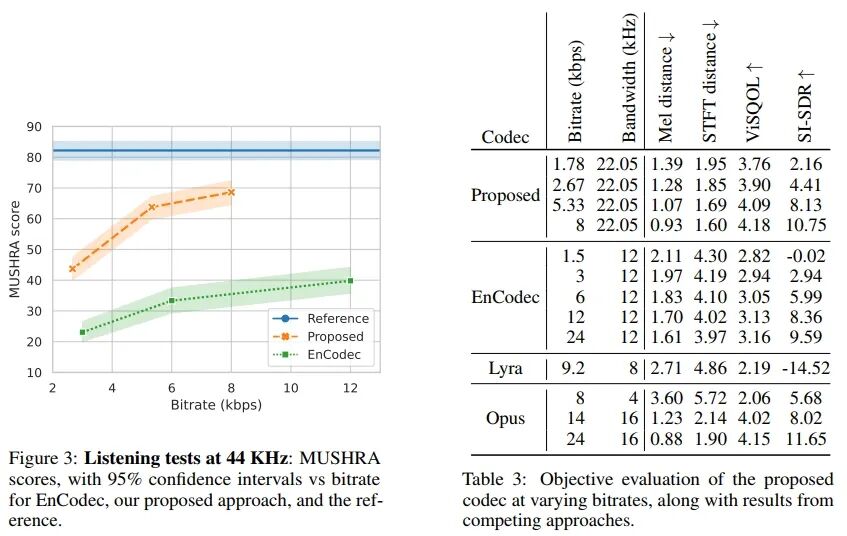

In Figure 3, we present our MUSHRA study results, which compare the performance of EnCodec with our proposed codec at different bitrates. We found that our codec received higher MUSHRA scores than EnCodec at all bitrates. However, even at the highest bitrate, it still failed to reach the reference MUSHRA score, indicating that there is still room for improvement. We noted that the metrics of our final model remain lower than those of the 24 kbps model we trained in the ablation study, as shown in Table 2. This suggests that the remaining performance gap may be narrowed by increasing the maximum bitrate.

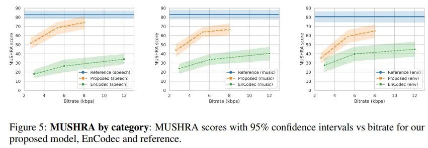
In Figure 4 and Table 4, we compare our proposed model trained with the exact same configuration as EnCodec (24 kHz sampling rate, 24 kbps bitrate, 320 stride, 32 codebooks of 10 bits each) with existing benchmark models in both quantitative and qualitative metrics. In Figure 5, we present qualitative results categorized by sound type.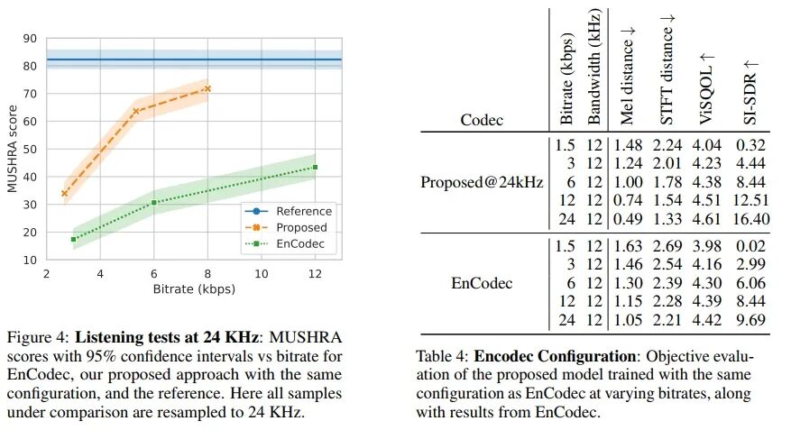

5 Conclusion

We proposed a high-fidelity universal neural audio compression algorithm that achieves significant compression rates while maintaining audio quality, suitable for various types of audio data. Our method combines the latest audio generation techniques, vector quantization techniques, and improved adversarial and reconstruction losses. Our extensive evaluation of existing audio compression algorithms demonstrates the superiority of our method, providing a promising foundation for future high-fidelity audio modeling. Through thorough ablation studies, open-source code, and trained model weights, we hope to make a valuable contribution to the generative audio modeling community.

Broader Implications and Limitations: Our model has the potential to make generative modeling of full-bandwidth audio easier. While this unlocks many useful applications such as media editing, text-to-speech synthesis, music synthesis, etc., it may also lead to harmful applications such as deepfakes. Caution is needed to avoid these applications. One possible measure is to add watermarks and/or train a classifier to detect whether this codec has been applied, so that synthetic media generated based on our codec can be detected. Additionally, our model is not perfect and still struggles with reconstructing some challenging audio. By breaking down results by domain, we found that while our proposed codec outperforms competing methods across all domains, it performs best in speech and has more issues with environmental audio. Finally, we note that it cannot perfectly model certain instruments, such as xylophones or synthesizer sounds.

Paper Title:
High-Fidelity Audio Compression with Improved RVQGAN
Paper Link:
https://proceedings.neurips.cc/paper_files/paper/2023/file/58d0e78cf042af5876e12661087bea12-Paper-Conference.pdf