Hello, everyone! I am the evolving ape, a learner exploring the field of data analysis. Today, we will continue our study of clustering analysis.
Clustering Effect Evaluation Metrics
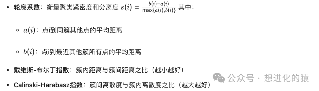
Internal Metrics (No True Labels Required)
External Metrics (True Labels Required)
- Adjusted Rand Index: Measures the similarity between clustering and true labels
- Mutual Information Score: Measures the mutual information between two label distributions
Evaluation Implementation and Interpretation
from sklearn.metrics import (    silhouette_score, davies_bouldin_score,     calinski_harabasz_score, adjusted_rand_score)from sklearn.datasets import load_irisfrom sklearn.cluster import AgglomerativeClusteringimport pandas as pd
# Load dataset with true labelsiris = load_iris()X_iris = iris.datay_iris = iris.target
# Standardize dataX_iris_scaled = StandardScaler().fit_transform(X_iris)
# Compare different clustering algorithmsmethods = {    'KMeans': KMeans(n_clusters=3, random_state=42),    'Agglomerative': AgglomerativeClustering(n_clusters=3),    'DBSCAN': DBSCAN(eps=0.7, min_samples=5)}results = []
for name, model in methods.items():    # Train clustering model    if name == 'DBSCAN':        labels = model.fit_predict(X_iris_scaled)        # Skip noise points calculation        valid_mask = labels != -1        if np.sum(valid_mask) == 0:            continue        filtered_labels = labels[valid_mask]        filtered_data = X_iris_scaled[valid_mask]        filtered_target = y_iris[valid_mask]    else:        labels = model.fit_predict(X_iris_scaled)        filtered_labels = labels        filtered_data = X_iris_scaled        filtered_target = y_iris
    # Calculate internal metrics    sil_score = silhouette_score(filtered_data, filtered_labels)    db_score = davies_bouldin_score(filtered_data, filtered_labels)    ch_score = calinski_harabasz_score(filtered_data, filtered_labels)
    # Calculate external metrics    ar_score = adjusted_rand_score(filtered_target, filtered_labels)
    # Save results    results.append({        'Method': name,        'Silhouette': sil_score,        'Davies-Bouldin': db_score,        'Calinski-Harabasz': ch_score,        'Adjusted Rand': ar_score,        'Clusters': len(np.unique(filtered_labels))    })
# Create results DataFrameresults_df = pd.DataFrame(results)print("\nClustering Algorithm Performance Comparison:")print(results_df)
# Visualize metric comparisonsfig, axes = plt.subplots(2, 2, figsize=(15, 10))metrics = ['Silhouette', 'Davies-Bouldin', 'Calinski-Harabasz', 'Adjusted Rand']titles = ['Silhouette Coefficient (Higher is Better)', 'Davies-Bouldin Index (Lower is Better)',           'Calinski-Harabasz Index (Higher is Better)', 'Adjusted Rand Index (Higher is Better)']
for i, metric in enumerate(metrics):    ax = axes[i//2, i%2]    sorted_df = results_df.sort_values(metric, ascending=(metric=='Davies-Bouldin'))    ax.bar(sorted_df['Method'], sorted_df[metric], color=['blue', 'green', 'red'])
    # Add value labels    for j, value in enumerate(sorted_df[metric]):        ax.text(j, value + 0.01, f'{value:.3f}', ha='center')    ax.set_title(titles[i])    ax.grid(axis='y')    if metric == 'Davies-Bouldin':        ax.set_ylim(0, sorted_df[metric].max() + 0.5)plt.tight_layout()plt.show()
The output results are as follows: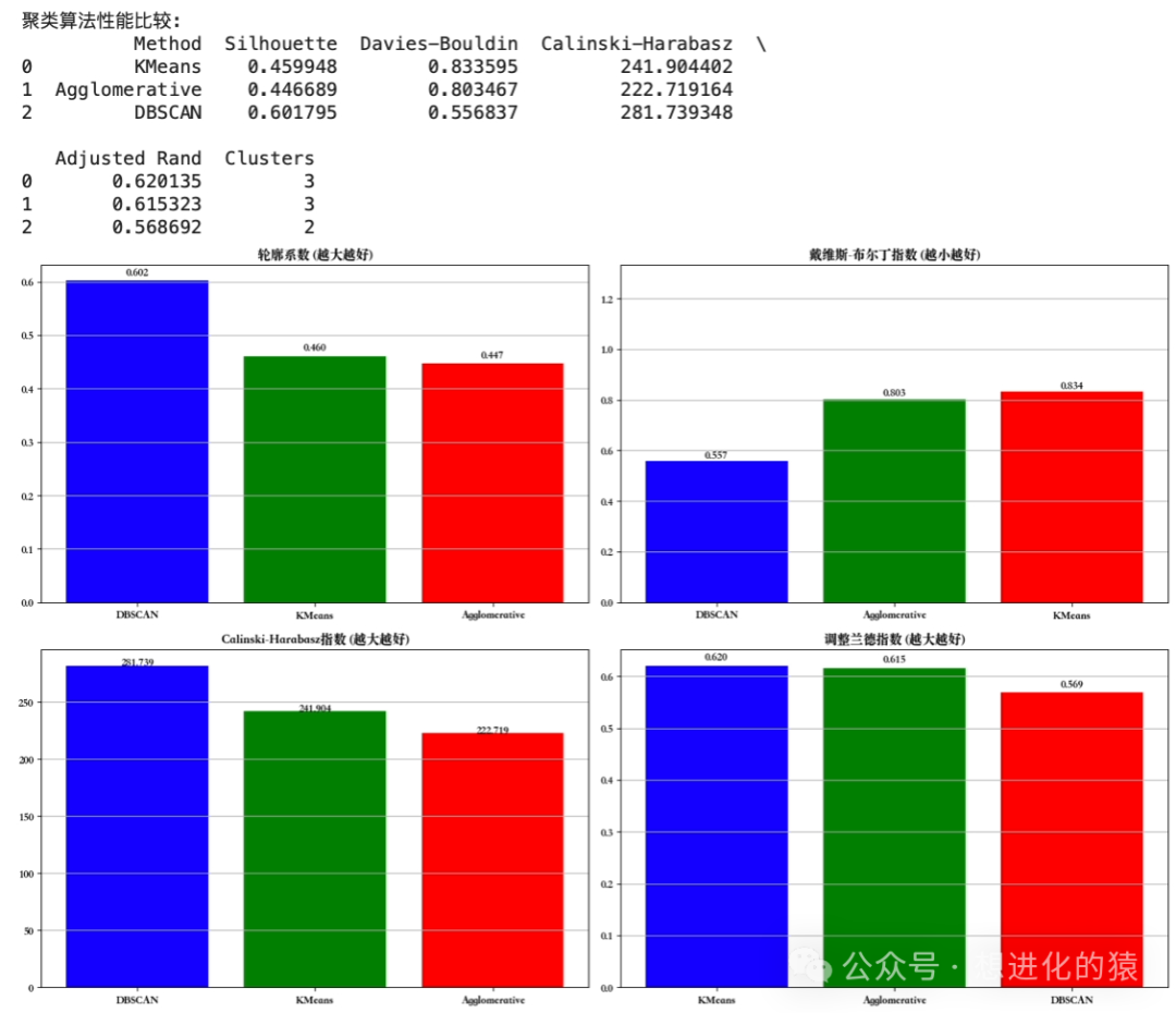
Methods for Determining the Number of Clusters
Elbow Method
Determine the optimal K value by observing the change in within-cluster sum of squares (WCSS) for different K values
from sklearn.metrics import pairwise_distances
# Implementation of Elbow Methoddef elbow_method(X, max_k=10):    wcss = []    silhouette_scores = []    k_range = range(1, max_k+1)
    for k in k_range:        # Skip the case for k=1        if k == 1:            wcss.append(0)            silhouette_scores.append(0)            continue
        kmeans = KMeans(n_clusters=k, random_state=42)        kmeans.fit(X)
        # Calculate within-cluster sum of squares        wcss.append(kmeans.inertia_)
        # Calculate silhouette coefficient        if k > 1:            silhouette_scores.append(silhouette_score(X, kmeans.labels_))        else:            silhouette_scores.append(0)
    # Find the elbow point (point of maximum curvature)    differences = np.diff(wcss)    second_derivatives = np.diff(differences)    elbow_index = np.argmin(second_derivatives) + 2  # Compensate for two differences
    # Visualization    plt.figure(figsize=(15, 6))
    # WCSS plot    plt.subplot(1, 2, 1)    plt.plot(k_range, wcss, 'bo-')    plt.xlabel('Number of Clusters K')    plt.ylabel('Within-Cluster Sum of Squares (WCSS)')    plt.title('Elbow Method')    plt.axvline(x=elbow_index, color='r', linestyle='--',                 label=f'Suggested K value={elbow_index}')    plt.xticks(k_range)    plt.grid(True)    plt.legend()
    # Silhouette coefficient plot    plt.subplot(1, 2, 2)    plt.plot(k_range[1:], silhouette_scores[1:], 'go-')    plt.xlabel('Number of Clusters K')    plt.ylabel('Silhouette Coefficient')    plt.title('Silhouette Coefficient Method')    max_sil_index = np.argmax(silhouette_scores[1:]) + 1    plt.axvline(x=max_sil_index, color='r', linestyle='--',                 label=f'Optimal K value={max_sil_index}')    plt.xticks(k_range[1:])    plt.grid(True)    plt.legend()
    plt.tight_layout()    plt.show()    return elbow_index, max_sil_index
# Apply Elbow Methodelbow_k, sil_k = elbow_method(X_scaled, max_k=10)print(f"Elbow Method Suggested K value: {elbow_k}")print(f"Silhouette Coefficient Method Suggested K value: {sil_k}")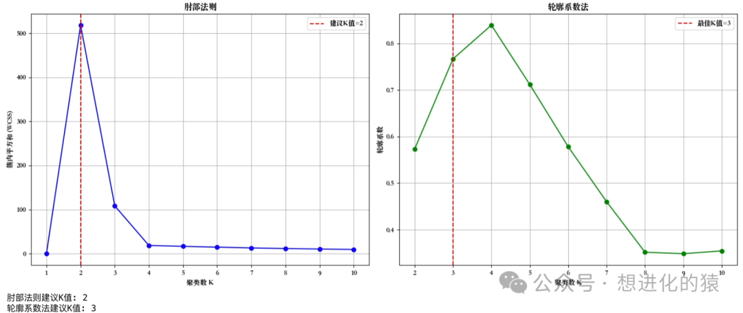
Silhouette Coefficient Method
Select the K value that maximizes the silhouette coefficient (already implemented above)
Gap Statistic
Compare the WCSS difference between actual data and uniformly distributed reference data
from gap_stat import OptimalK  # pip install gap-stat

def gap_statistic(X, max_k=10):    """Determine the optimal number of clusters using Gap Statistic"""    optimalK = OptimalK(parallel_backend='rust')  # Use Rust backend for accelerated computation    n_clusters = optimalK(X, cluster_array=range(1, max_k+1))
    # Visualize results    plt.figure(figsize=(10, 6))    optimalK.plot_results()    plt.title('Gap Statistic')    plt.xlabel('Number of Clusters K')    plt.ylabel('Gap Value')    plt.grid(True)    plt.show()    return n_clusters
# Apply Gap Statisticgap_k = gap_statistic(X_scaled, max_k=10)print(f"Gap Statistic Suggested K value: {gap_k}")
Industrial Application: Customer Segmentation Practice
import pandas as pdimport seaborn as snsfrom sklearn.decomposition import PCA
# Load customer dataset# Dataset source: https://www.kaggle.com/datasets/vjchoudhary7/customer-segmentation-tutorial-in-pythoncustomer_df = pd.read_csv('Mall_Customers.csv')print(customer_df.head())
# Feature engineeringcustomer_df.rename(columns={    'Annual Income (k$)': 'Income',    'Spending Score (1-100)': 'SpendingScore',    'Age': 'Age'}, inplace=True)
# Select relevant featuresfeatures = ['Age', 'Income', 'SpendingScore']X_cust = customer_df[features]
# Standardize datascaler = StandardScaler()X_cust_scaled = scaler.fit_transform(X_cust)
# Determine optimal number of clusters (combined from three methods)elbow_k, sil_k, gap_k = 4, 5, 5  # In actual applications, calculate using the above methodsfinal_k = max(set([elbow_k, sil_k, gap_k]), key=[elbow_k, sil_k, gap_k].count)print(f"Comprehensive Suggested Number of Clusters: {final_k}")
# Use K-means clusteringcust_kmeans = KMeans(n_clusters=final_k, random_state=42)customer_df['Cluster'] = cust_kmeans.fit_predict(X_cust_scaled)
# Dimensionality reduction visualizationpca = PCA(n_components=2)X_pca = pca.fit_transform(X_cust_scaled)customer_df['PCA1'] = X_pca[:, 0]customer_df['PCA2'] = X_pca[:, 1]
# Visualize clustering resultsplt.figure(figsize=(12, 8))sns.scatterplot(    x='PCA1', y='PCA2',     hue='Cluster',     data=customer_df,    palette='viridis',    s=100,    alpha=0.8)plt.title('Customer Clustering Results (PCA Dimensionality Reduction)')plt.grid(True)plt.show()
# Analyze features of each clustercluster_summary = customer_df.groupby('Cluster')[features].mean()print("\nMean Feature Values for Each Cluster:")print(cluster_summary)
# Draw radar chart to display cluster featuresfig = plt.figure(figsize=(10, 8))ax = fig.add_subplot(111, polar=True)
# Calculate anglesangles = np.linspace(0, 2*np.pi, len(features), endpoint=False).tolist()angles += angles[:1]  # Close the shape
# Normalize feature valuessummary_normalized = cluster_summary.copy()for feature in features:    summary_normalized[feature] = (cluster_summary[feature] - cluster_summary[feature].min()) /
                                  (cluster_summary[feature].max() - cluster_summary[feature].min())# Draw radar chart for each clusterfor cluster in range(final_k):    values = summary_normalized.loc[cluster].values.tolist()    values += values[:1]  # Close the shape
    ax.plot(angles, values, 'o-', linewidth=2, label=f'Cluster {cluster}')    ax.fill(angles, values, alpha=0.25)
# Add labelsax.set_theta_offset(np.pi/2)ax.set_theta_direction(-1)ax.set_thetagrids(np.degrees(angles[:-1]), features)
# Add legendplt.legend(loc='upper right', bbox_to_anchor=(1.3, 1.1))plt.title('Radar Chart of Cluster Features')plt.grid(True)plt.show()
# Business interpretation and action recommendationscluster_profiles = {    0: "Moderate Income Young Consumers - Targeted Marketing",    1: "High Income Middle-aged Consumers - High-end Product Recommendations",    2: "Low Income Consumers - Discount Promotions",    3: "High Spending Young Groups - Trendy Product Promotion",    4: "Low Spending Elderly Groups - Basic Service Maintenance"}customer_df['ClusterProfile'] = customer_df['Cluster'].map(cluster_profiles)print("\nBusiness Interpretation and Action Recommendations for Each Cluster:", cluster_profiles)
Clustering Algorithm Selection Guide
| Scenario | Recommended Algorithm | Advantages | Considerations |
|---|---|---|---|
| Known Number of Clusters | K-Means | Computationally efficient, intuitive results | Sensitive to outliers, data needs to be standardized |
| Hierarchical Structure in Data | Hierarchical Clustering | Visualizable dendrogram, no need to preset K value | High computational complexity, O(n²) time complexity |
| Arbitrary Shaped Clusters | DBSCAN | Discovers arbitrary shaped clusters, identifies noise points | ε and min_samples parameters need tuning |
| High Dimensional Data | Spectral Clustering | Strong capability to handle high-dimensional data | Requires similarity matrix, high computational cost |
| Large Scale Data | Mini-Batch K-Means | Memory efficient, supports incremental learning | Accuracy slightly lower than standard K-Means |
Conclusion
- Data Preprocessing: Standardization/Normalization is Key (Except for DBSCAN)
- Multi-method Validation: Combine Elbow Method, Silhouette Coefficient, and Gap Statistic to Determine K Value
- Business Interpretation: The Key is to Assign Business Meaning to Clustering Results
- Feature Engineering: PCA Dimensionality Reduction to Visualize Clustering Results
- Model Monitoring: Regularly Re-cluster to Adapt to Data Changes
Clustering analysis, as a core method of unsupervised learning, is widely used in customer segmentation, anomaly detection, image segmentation, and other fields. Mastering the principles of different clustering algorithms and applicable scenarios, combined with business knowledge to interpret clustering results, can provide strong support for data-driven decision-making.