In-Depth Analysis of the C-MAPSS Dataset
The C-MAPSS dataset was developed by NASA for research on aircraft engine fault prediction. It is highly favored in the field of engine life prediction and frequently appears in various top journals. Due to its relatively complete data, ease of organization, and high difficulty in data fitting, it serves as a touchstone for testing the performance of deep learning algorithms. This article uses MATLAB code to conduct a deep analysis of this data.
1. Overview of the Dataset
C-MAPSS (Commercial Modular Aero-Propulsion System Simulation) is a simulation dataset for aircraft engine degradation, with the official data access link:https://data.nasa.gov/dataset/cmapss-jet-engine-simulated-data
The C-MAPSS dataset consists of four independent subsets (FD001-FD004), each designed for different operating conditions and fault scenarios, with the specific configurations as follows:
| Subset | Number of Training Samples | Number of Testing Samples | Operating Conditions | Fault Modes |
|---|---|---|---|---|
| FD001 | 100 | 100 | Single Condition | High Pressure Compressor (HPC) Degradation |
| FD002 | 260 | 259 | Six Mixed Conditions | HPC Degradation |
| FD003 | 100 | 100 | Single Condition | HPC + Fan Composite Degradation |
| FD004 | 248 | 249 | Six Mixed Conditions | HPC + Fan Composite Degradation |
FD001/FD003 focus on single conditions, while FD002/FD004 simulate complex scenarios with multiple condition switches. FD003/FD004 additionally introduce fan degradation issues.
Taking FD001 as an example, the training trajectory refers to the time series data of each engine during its operational cycle. Each training trajectory corresponds to the operational data of one engine. 100 training trajectories represent 100 engines, each with different initial wear and manufacturing processes, which are considered normal variations rather than fault conditions.
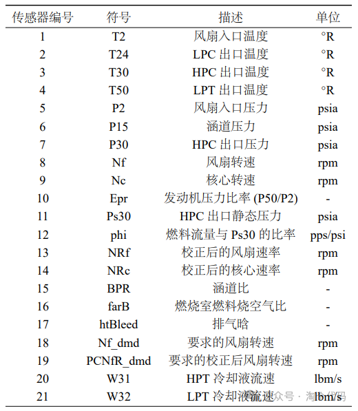
The dataset contains values recorded by 21 sensors and different operational settings, which significantly impact engine performance.
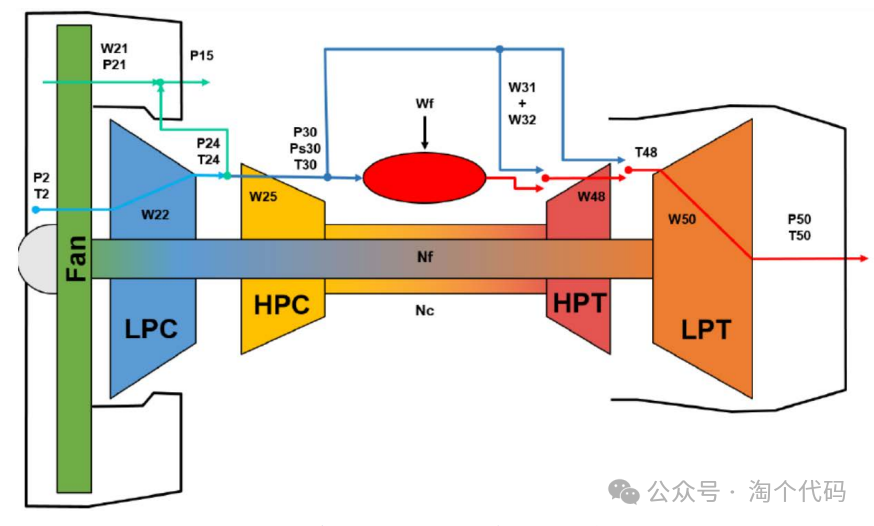
- Physical Meaning of the C-MAPSS Dataset
- Sensor Distribution as shown:
 In the training set, the simulated engine undergoes a complete degradation process from a healthy state to a fault state; while in the testing set, partial degradation trajectories of some engines are provided, with data randomly truncated before the actual fault occurrence (i.e., not reaching the true fault time point). The testing model infers the remaining useful life based on the current sensor values.
2. Deep Analysis of Data with MATLAB Code
Loading C-MAPSS Data:
% Core code for data loading
clear; clc; close all;
addpath(genpath(pwd)); % Add current directory to path

% Define function to read data
function data = get_data(file_name)
    file_path = fullfile('C-MAPSS-Data\', file_name);
    if exist(file_path, 'file') == 2
        data = readtable(file_path, 'Delimiter', ' ', 'MultipleDelimsAsOne', true, ...
            'ReadVariableNames', false,'HeaderLines', 0);
    else
        error('File not found: %s', file_path);
    end
end
%% Load all datasets
% Training data
train_FD001 = get_data('train_FD001.txt');
train_FD002 = get_data('train_FD002.txt');
train_FD003 = get_data('train_FD003.txt');
train_FD004 = get_data('train_FD004.txt');

% RUL data
RUL_FD001 = get_data('RUL_FD001.txt');
RUL_FD002 = get_data('RUL_FD002.txt');
RUL_FD003 = get_data('RUL_FD003.txt');
RUL_FD004 = get_data('RUL_FD004.txt');

% Testing data
test_FD001 = get_data('test_FD001.txt');
test_FD002 = get_data('test_FD002.txt');
test_FD003 = get_data('test_FD003.txt');
test_FD004 = get_data('test_FD004.txt');

%% Set column names
col_names = {'ID', 'cycle', 'op_set_1', 'op_set_2', 'op_set_3', ...
    'sensor_1', 'sensor_2', 'sensor_3', 'sensor_4', 'sensor_5', ...
    'sensor_6', 'sensor_7', 'sensor_8', 'sensor_9', 'sensor_10', ...
    'sensor_11', 'sensor_12', 'sensor_13', 'sensor_14', 'sensor_15', ...
    'sensor_16', 'sensor_17', 'sensor_18', 'sensor_19', 'sensor_20', ...
    'sensor_21'};
col_name_RUL = {'RUL'};

% Assign column names to all datasets
datasets = {train_FD001, train_FD002, train_FD003, train_FD004, ...
    test_FD001, test_FD002, test_FD003, test_FD004, ...
    RUL_FD001, RUL_FD002, RUL_FD003, RUL_FD004};

col_sets = {repmat({col_names}, 1, 8), repmat({col_name_RUL}, 1, 4)};

for i = 1:12
    if i <= 8
        datasets{i}.Properties.VariableNames = col_names;
    else
        datasets{i}.Properties.VariableNames = col_name_RUL;
    end
end
% Assign updated datasets back to original variables
train_FD001 = datasets{1};
train_FD002 = datasets{2};
train_FD003 = datasets{3};
train_FD004 = datasets{4};

test_FD001 = datasets{5};
test_FD002 = datasets{6};
test_FD003 = datasets{7};
test_FD004 = datasets{8};

RUL_FD001 = datasets{9};
RUL_FD002 = datasets{10};
RUL_FD003 = datasets{11};
RUL_FD004 = datasets{12};
Data Quality Check:
% Check for null values
fprintf('Null value check:\n');
for i = 1:8
    null_count = sum(any(ismissing(datasets{i}), 1));
    fprintf('Dataset %d: %d null values\n', i, null_count);
end

% Check for duplicate values
fprintf('\nDuplicate value check:\n');
for i = 1:8
    [~, idx] = unique(datasets{i}, 'rows');
    dup_count = size(datasets{i}, 1) - length(idx);
    fprintf('Dataset %d: %d duplicate values\n', i, dup_count);
end
MATLAB output as follows: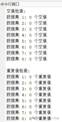
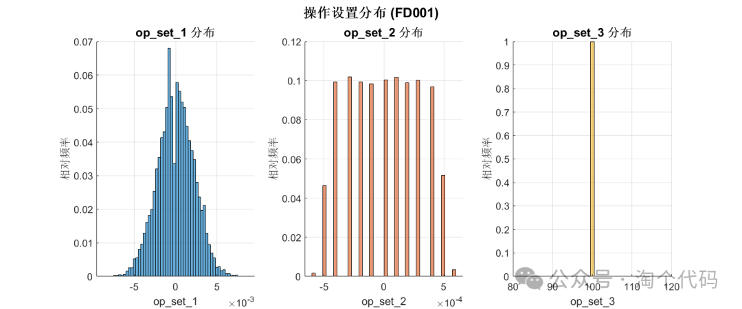
Operating Settings Distribution Chart:
%% Create unified plotting style
myColors = [0 0.4470 0.7410; 0.8500 0.3250 0.0980; 0.9290 0.6940 0.1250; ...
    0.4940 0.1840 0.5560; 0.4660 0.6740 0.1880; 0.3010 0.7450 0.9330; ...
    0.6350 0.0780 0.1840];
set(groot, 'defaultFigureColor', 'white', ...
    'defaultAxesFontSize', 12, ...
    'defaultAxesLabelFontSizeMultiplier', 1.1, ...
    'defaultAxesTitleFontSizeMultiplier', 1.2, ...
    'defaultLineLineWidth', 1.5);

%% Operating Settings Analysis (FD001)
% Extract operating settings columns
op_set_cols = contains(col_names, 'op_set');
op_set_names = col_names(op_set_cols);

% Histogram distribution
figure('Position', [100, 100, 1200, 500]);
for i = 1:3
    subplot(1, 3, i);
    data = train_FD001.(op_set_names{i});
histogram(data, 'Normalization', 'probability', ...
        'FaceColor', myColors(i, :));
    title(sprintf('%s Distribution', op_set_names{i}), 'FontWeight', 'bold', 'Interpreter', 'none');
    xlabel(op_set_names{i},'Interpreter', 'none');
    ylabel('Relative Frequency');
    grid on;
    box off;
    if i==3
        xlim([80, 120]); % Manually set x-axis range
    end
end
sgtitle('Operating Settings Distribution (FD001)', 'FontSize', 16, 'FontWeight', 'bold');
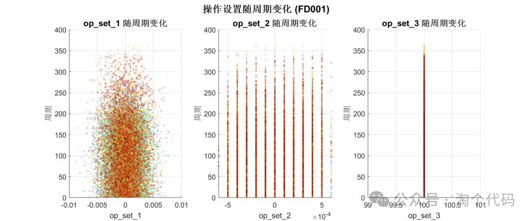
Operating Settings Change Over Cycles:
% Operating settings change over cycles
figure('Position', [100, 100, 1200, 500]);
for i = 1:3
    subplot(1, 3, i);
    scatter(train_FD001.(op_set_names{i}), train_FD001.cycle, 8, ...
        train_FD001.ID, 'filled', 'MarkerEdgeAlpha', 0.3, 'MarkerFaceAlpha', 0.3);
    title(sprintf('%s Change Over Cycles', op_set_names{i}), 'FontWeight', 'bold', 'Interpreter', 'none');
    xlabel(op_set_names{i}, 'Interpreter', 'none');
    ylabel('Cycle');
    colormap(turbo);
    colorbar('off');
    grid on;
end
sgtitle('Operating Settings Change Over Cycles (FD001)', 'FontSize', 16, 'FontWeight', 'bold');
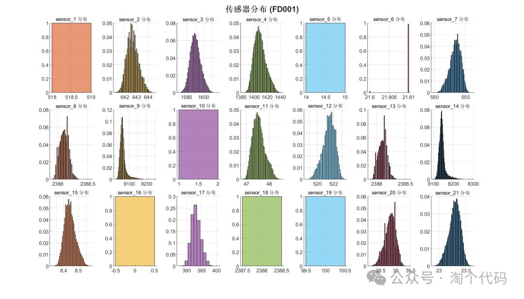
Sensor Analysis (FD001)
Taking FD001 as an example:
% Extract sensor columns
sensor_cols = contains(col_names, 'sensor');
sensor_names = col_names(sensor_cols);

% Sensor histogram
figure('Position', [100, 100, 1400, 800]);
tiledlayout(3, 7, 'TileSpacing', 'compact');
for i = 1:21
    nexttile;
    data = train_FD001.(sensor_names{i});
histogram(data, 'Normalization', 'probability', ...
        'FaceColor', myColors(mod(i,7)+1, :));
    title(sprintf('%s Distribution', sensor_names{i}), 'FontSize', 10, 'Interpreter', 'none');
    grid on;
    box off;
end
sgtitle('Sensor Distribution (FD001)', 'FontSize', 16, 'FontWeight', 'bold');
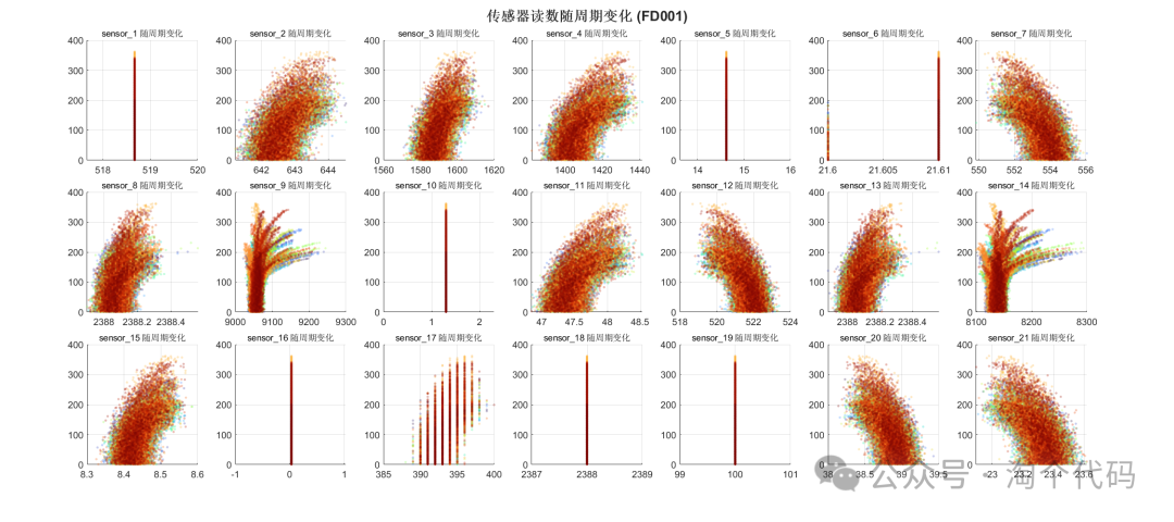
Sensor Change Over Cycles
% Sensor change over cycles
figure('Position', [100, 100, 1800, 800]);
tiledlayout(3, 7, 'TileSpacing', 'compact');
for i = 1:21
    nexttile;
    scatter(train_FD001.(sensor_names{i}), train_FD001.cycle, 8, ...
        train_FD001.ID, 'filled', 'MarkerEdgeAlpha', 0.3, 'MarkerFaceAlpha', 0.3);
    title(sprintf('%s Change Over Cycles', sensor_names{i}), 'FontSize', 10, 'Interpreter', 'none');
    colormap(turbo);
    colorbar('off');
    grid on;
end
sgtitle('Sensor Readings Change Over Cycles (FD001)', 'FontSize', 16, 'FontWeight', 'bold');
Relationship Between Operating Settings and RUL (Remaining Useful Life)
%% Calculate RUL (FD001)
% Calculate the maximum cycle for each engine
[G, ID_groups] = findgroups(train_FD001.ID);
max_cycle = splitapply(@max, train_FD001.cycle, G);
max_cycle_per_engine = table(ID_groups, max_cycle, 'VariableNames', {'ID', 'max_cycle'});

% Merge data and calculate RUL
train_FD001_merged = join(train_FD001, max_cycle_per_engine);
train_FD001_merged.RUL = train_FD001_merged.max_cycle - train_FD001_merged.cycle;

%% RUL Analysis (FD001)
% Relationship between operating settings and RUL
figure('Position', [100, 100, 1200, 500]);
for i = 1:3
    subplot(1, 3, i);
    scatter(train_FD001_merged.(op_set_names{i}), train_FD001_merged.RUL, 8, ...
        train_FD001_merged.ID, 'filled', 'MarkerEdgeAlpha', 0.3, 'MarkerFaceAlpha', 0.3);
    title(sprintf('%s Relationship with RUL', op_set_names{i}), 'FontWeight', 'bold', 'Interpreter', 'none');
    xlabel(op_set_names{i}, 'Interpreter', 'none');
    ylabel('RUL');
    colormap(turbo);
    colorbar('off');
    grid on;
end
sgtitle('Operating Settings and RUL Relationship (FD001)', 'FontSize', 16, 'FontWeight', 'bold');

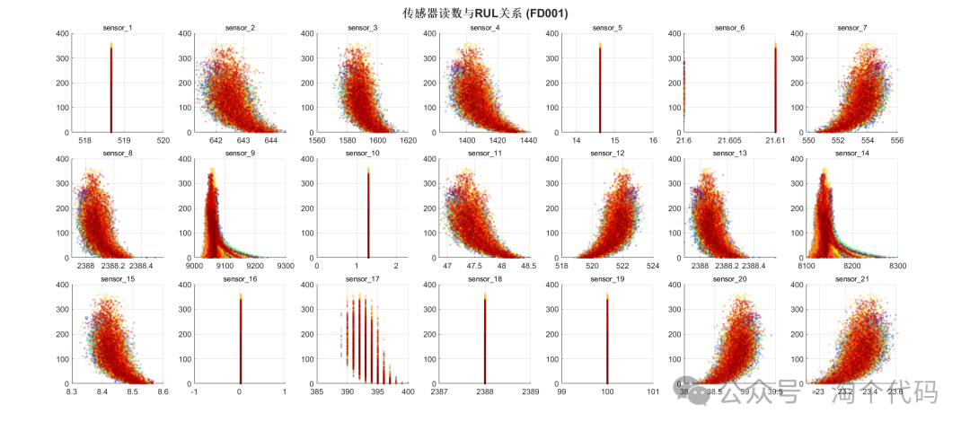
Relationship Between Sensors and RUL
% Relationship between sensors and RUL
figure('Position', [100, 100, 1800, 800]);
colormap(jet);                    % Use clearer color schemes (e.g., parula, jet, hsv)
tiledlayout(3, 7, 'TileSpacing', 'compact');
for i = 1:21
    nexttile;
    scatter(train_FD001_merged.(sensor_names{i}), train_FD001_merged.RUL, 8, ...
        train_FD001_merged.ID, 'filled', 'MarkerEdgeAlpha', 0.3, 'MarkerFaceAlpha', 0.3);
    title(sensor_names{i}, 'FontSize', 10, 'Interpreter', 'none');
    grid on;
end
sgtitle('Sensor Readings and RUL Relationship (FD001)', 'FontSize', 16, 'FontWeight', 'bold');
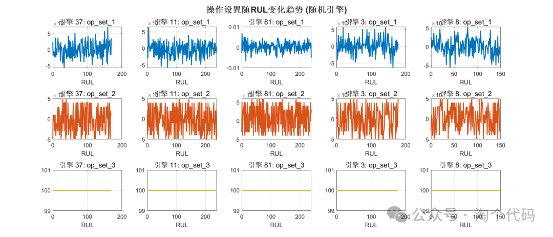
Random Selection of 5 Engines for Trend Analysis
- Trend of Operating Settings with RUL
engine_ids = randperm(100, 5); % Randomly select 5 engines

% Operating settings trend analysis
figure('Position', [100, 100, 1400, 600]);
tiledlayout(3, 5, 'TileSpacing', 'compact');
for i = 1:3
    for j = 1:5
        nexttile;
        engine_data = train_FD001_merged(train_FD001_merged.ID == engine_ids(j), :);
        plot(engine_data.RUL, engine_data.(op_set_names{i}), ...
            'Color', myColors(i, :), 'LineWidth', 1.8);
        title(sprintf('Engine %d: %s', engine_ids(j), op_set_names{i}), 'Interpreter', 'none');
        xlabel('RUL', 'Interpreter', 'none');
        grid on;
    end
end
sgtitle('Trend of Operating Settings with RUL (Random Engines)', 'FontSize', 16, 'FontWeight', 'bold');
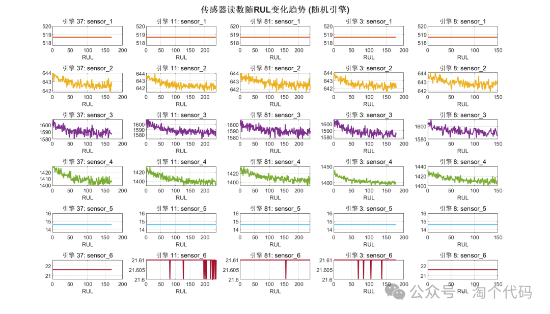
- Trend of Sensors with RUL
sensor_subset = sensor_names(1:6);
figure('Position', [100, 100, 1400, 800]);
tiledlayout(6, 5, 'TileSpacing', 'compact');
for i = 1:6
    for j = 1:5
        nexttile;
        engine_data = train_FD001_merged(train_FD001_merged.ID == engine_ids(j), :);
        plot(engine_data.RUL, engine_data.(sensor_subset{i}), ...
            'Color', myColors(mod(i,7)+1, :), 'LineWidth', 1.8);
        title(sprintf('Engine %d: %s', engine_ids(j), sensor_subset{i}), 'Interpreter', 'none');
        xlabel('RUL');
        grid on;
    end
end
sgtitle('Sensor Readings Trend with RUL (Random Engines)', 'FontSize', 16, 'FontWeight', 'bold');
3. Complete Code for Direct Copy
%% Initialize Environment
clear; clc; close all;
addpath(genpath(pwd)); % Add current directory to path

% Define function to read data
function data = get_data(file_name)
    file_path = fullfile('C-MAPSS-Data\', file_name);
    if exist(file_path, 'file') == 2
        data = readtable(file_path, 'Delimiter', ' ', 'MultipleDelimsAsOne', true, ...
            'ReadVariableNames', false,'HeaderLines', 0);
    else
        error('File not found: %s', file_path);
    end
end
%% Load all datasets
% Training data
train_FD001 = get_data('train_FD001.txt');
train_FD002 = get_data('train_FD002.txt');
train_FD003 = get_data('train_FD003.txt');
train_FD004 = get_data('train_FD004.txt');

% RUL data
RUL_FD001 = get_data('RUL_FD001.txt');
RUL_FD002 = get_data('RUL_FD002.txt');
RUL_FD003 = get_data('RUL_FD003.txt');
RUL_FD004 = get_data('RUL_FD004.txt');

% Testing data
test_FD001 = get_data('test_FD001.txt');
test_FD002 = get_data('test_FD002.txt');
test_FD003 = get_data('test_FD003.txt');
test_FD004 = get_data('test_FD004.txt');

%% Set column names
col_names = {'ID', 'cycle', 'op_set_1', 'op_set_2', 'op_set_3', ...
    'sensor_1', 'sensor_2', 'sensor_3', 'sensor_4', 'sensor_5', ...
    'sensor_6', 'sensor_7', 'sensor_8', 'sensor_9', 'sensor_10', ...
    'sensor_11', 'sensor_12', 'sensor_13', 'sensor_14', 'sensor_15', ...
    'sensor_16', 'sensor_17', 'sensor_18', 'sensor_19', 'sensor_20', ...
    'sensor_21'};
col_name_RUL = {'RUL'};

% Assign column names to all datasets
datasets = {train_FD001, train_FD002, train_FD003, train_FD004, ...
    test_FD001, test_FD002, test_FD003, test_FD004, ...
    RUL_FD001, RUL_FD002, RUL_FD003, RUL_FD004};

col_sets = {repmat({col_names}, 1, 8), repmat({col_name_RUL}, 1, 4)};

for i = 1:12
    if i <= 8
        datasets{i}.Properties.VariableNames = col_names;
    else
        datasets{i}.Properties.VariableNames = col_name_RUL;
    end
end
% Assign updated datasets back to original variables
train_FD001 = datasets{1};
train_FD002 = datasets{2};
train_FD003 = datasets{3};
train_FD004 = datasets{4};

test_FD001 = datasets{5};
test_FD002 = datasets{6};
test_FD003 = datasets{7};
test_FD004 = datasets{8};

RUL_FD001 = datasets{9};
RUL_FD002 = datasets{10};
RUL_FD003 = datasets{11};
RUL_FD004 = datasets{12};

%% Data Quality Check
% Check for null values
fprintf('Null value check:\n');
for i = 1:8
    null_count = sum(any(ismissing(datasets{i}), 1));
    fprintf('Dataset %d: %d null values\n', i, null_count);
end

% Check for duplicate values
fprintf('\nDuplicate value check:\n');
for i = 1:8
    [~, idx] = unique(datasets{i}, 'rows');
    dup_count = size(datasets{i}, 1) - length(idx);
    fprintf('Dataset %d: %d duplicate values\n', i, dup_count);
end

%% Create unified plotting style
myColors = [0 0.4470 0.7410; 0.8500 0.3250 0.0980; 0.9290 0.6940 0.1250; ...
    0.4940 0.1840 0.5560; 0.4660 0.6740 0.1880; 0.3010 0.7450 0.9330; ...
    0.6350 0.0780 0.1840];
set(groot, 'defaultFigureColor', 'white', ...
    'defaultAxesFontSize', 12, ...
    'defaultAxesLabelFontSizeMultiplier', 1.1, ...
    'defaultAxesTitleFontSizeMultiplier', 1.2, ...
    'defaultLineLineWidth', 1.5);

%% Operating Settings Analysis (FD001)
% Extract operating settings columns
op_set_cols = contains(col_names, 'op_set');
op_set_names = col_names(op_set_cols);

% Histogram distribution
figure('Position', [100, 100, 1200, 500]);
for i = 1:3
    subplot(1, 3, i);
    data = train_FD001.(op_set_names{i});
histogram(data, 'Normalization', 'probability', ...
        'FaceColor', myColors(i, :));
    title(sprintf('%s Distribution', op_set_names{i}), 'FontWeight', 'bold', 'Interpreter', 'none');
    xlabel(op_set_names{i},'Interpreter', 'none');
    ylabel('Relative Frequency');
    grid on;
    box off;
    if i==3
        xlim([80, 120]); % Manually set x-axis range
    end
end
sgtitle('Operating Settings Distribution (FD001)', 'FontSize', 16, 'FontWeight', 'bold');

% Operating settings change over cycles
figure('Position', [100, 100, 1200, 500]);
for i = 1:3
    subplot(1, 3, i);
    scatter(train_FD001.(op_set_names{i}), train_FD001.cycle, 8, ...
        train_FD001.ID, 'filled', 'MarkerEdgeAlpha', 0.3, 'MarkerFaceAlpha', 0.3);
    title(sprintf('%s Change Over Cycles', op_set_names{i}), 'FontWeight', 'bold', 'Interpreter', 'none');
    xlabel(op_set_names{i}, 'Interpreter', 'none');
    ylabel('Cycle');
    colormap(turbo);
    colorbar('off');
    grid on;
end
sgtitle('Operating Settings Change Over Cycles (FD001)', 'FontSize', 16, 'FontWeight', 'bold');

%% Sensor Analysis (FD001)
% Extract sensor columns
sensor_cols = contains(col_names, 'sensor');
sensor_names = col_names(sensor_cols);

% Sensor histogram
figure('Position', [100, 100, 1400, 800]);
tiledlayout(3, 7, 'TileSpacing', 'compact');
for i = 1:21
    nexttile;
    data = train_FD001.(sensor_names{i});
histogram(data, 'Normalization', 'probability', ...
        'FaceColor', myColors(mod(i,7)+1, :));
    title(sprintf('%s Distribution', sensor_names{i}), 'FontSize', 10, 'Interpreter', 'none');
    grid on;
    box off;
end
sgtitle('Sensor Distribution (FD001)', 'FontSize', 16, 'FontWeight', 'bold');

% Sensor change over cycles
figure('Position', [100, 100, 1800, 800]);
tiledlayout(3, 7, 'TileSpacing', 'compact');
for i = 1:21
    nexttile;
    scatter(train_FD001.(sensor_names{i}), train_FD001.cycle, 8, ...
        train_FD001.ID, 'filled', 'MarkerEdgeAlpha', 0.3, 'MarkerFaceAlpha', 0.3);
    title(sprintf('%s Change Over Cycles', sensor_names{i}), 'FontSize', 10, 'Interpreter', 'none');
    colormap(turbo);
    colorbar('off');
    grid on;
end
sgtitle('Sensor Readings Change Over Cycles (FD001)', 'FontSize', 16, 'FontWeight', 'bold');

%% Calculate RUL (FD001)
% Calculate the maximum cycle for each engine
[G, ID_groups] = findgroups(train_FD001.ID);
max_cycle = splitapply(@max, train_FD001.cycle, G);
max_cycle_per_engine = table(ID_groups, max_cycle, 'VariableNames', {'ID', 'max_cycle'});

% Merge data and calculate RUL
train_FD001_merged = join(train_FD001, max_cycle_per_engine);
train_FD001_merged.RUL = train_FD001_merged.max_cycle - train_FD001_merged.cycle;

%% RUL Analysis (FD001)
% Relationship between operating settings and RUL
figure('Position', [100, 100, 1200, 500]);
for i = 1:3
    subplot(1, 3, i);
    scatter(train_FD001_merged.(op_set_names{i}), train_FD001_merged.RUL, 8, ...
        train_FD001_merged.ID, 'filled', 'MarkerEdgeAlpha', 0.3, 'MarkerFaceAlpha', 0.3);
    title(sprintf('%s Relationship with RUL', op_set_names{i}), 'FontWeight', 'bold', 'Interpreter', 'none');
    xlabel(op_set_names{i}, 'Interpreter', 'none');
    ylabel('RUL');
    colormap(turbo);
    colorbar('off');
    grid on;
end
sgtitle('Operating Settings and RUL Relationship (FD001)', 'FontSize', 16, 'FontWeight', 'bold');

% Relationship between sensors and RUL
figure('Position', [100, 100, 1800, 800]);
colormap(jet);                    % Use clearer color schemes (e.g., parula, jet, hsv)
tiledlayout(3, 7, 'TileSpacing', 'compact');
for i = 1:21
    nexttile;
    scatter(train_FD001_merged.(sensor_names{i}), train_FD001_merged.RUL, 8, ...
        train_FD001_merged.ID, 'filled', 'MarkerEdgeAlpha', 0.3, 'MarkerFaceAlpha', 0.3);
    title(sensor_names{i}, 'FontSize', 10, 'Interpreter', 'none');
    grid on;
end
sgtitle('Sensor Readings and RUL Relationship (FD001)', 'FontSize', 16, 'FontWeight', 'bold');

%% Correlation Analysis (FD001)
% Extract relevant columns
corr_cols = contains(train_FD001_merged.Properties.VariableNames, ...
    {'op_set', 'sensor', 'RUL'}) | ...
    strcmp(train_FD001_merged.Properties.VariableNames, 'cycle');
corr_data = train_FD001_merged(:, corr_cols);

% Calculate and display correlation coefficient matrix
corr_matrix = corr(table2array(corr_data), 'Rows', 'complete');
figure('Position', [100, 100, 1000, 900]);
imagesc(corr_matrix);
colorbar;
% colormap(jet);
title('Feature Correlation Matrix (FD001)', 'FontSize', 16, 'FontWeight', 'bold');
axis square;

%% Random Selection of 5 Engines for Trend Analysis
engine_ids = randperm(100, 5); % Randomly select 5 engines

% Operating settings trend analysis
figure('Position', [100, 100, 1400, 600]);
tiledlayout(3, 5, 'TileSpacing', 'compact');
for i = 1:3
    for j = 1:5
        nexttile;
        engine_data = train_FD001_merged(train_FD001_merged.ID == engine_ids(j), :);
        plot(engine_data.RUL, engine_data.(op_set_names{i}), ...
            'Color', myColors(i, :), 'LineWidth', 1.8);
        title(sprintf('Engine %d: %s', engine_ids(j), op_set_names{i}), 'Interpreter', 'none');
        xlabel('RUL', 'Interpreter', 'none');
        grid on;
    end
end
sgtitle('Trend of Operating Settings with RUL (Random Engines)', 'FontSize', 16, 'FontWeight', 'bold');

% Sensor trend analysis (selecting first 6 sensors as examples)
sensor_subset = sensor_names(1:6);
figure('Position', [100, 100, 1400, 800]);
tiledlayout(6, 5, 'TileSpacing', 'compact');
for i = 1:6
    for j = 1:5
        nexttile;
        engine_data = train_FD001_merged(train_FD001_merged.ID == engine_ids(j), :);
        plot(engine_data.RUL, engine_data.(sensor_subset{i}), ...
            'Color', myColors(mod(i,7)+1, :), 'LineWidth', 1.8);
        title(sprintf('Engine %d: %s', engine_ids(j), sensor_subset{i}), 'Interpreter', 'none');
        xlabel('RUL');
        grid on;
    end
end
sgtitle('Sensor Readings Trend with RUL (Random Engines)', 'FontSize', 16, 'FontWeight', 'bold');

%% Process FD002 Dataset (Example)
[G, ID_groups] = findgroups(train_FD002.ID);
max_cycle = splitapply(@max, train_FD002.cycle, G);
max_cycle_per_engine = table(ID_groups, max_cycle, 'VariableNames', {'ID', 'max_cycle'});

train_FD002_merged = join(train_FD002, max_cycle_per_engine);
train_FD002_merged.RUL = train_FD002_merged.max_cycle - train_FD002_merged.cycle;

% Relationship between operating settings and RUL
figure('Position', [100, 100, 1200, 500]);
for i = 1:3
    subplot(1, 3, i);
    scatter(train_FD002_merged.(op_set_names{i}), train_FD002_merged.RUL, 8, ...
        train_FD002_merged.ID, 'filled', 'MarkerEdgeAlpha', 0.3, 'MarkerFaceAlpha', 0.3);
    title(sprintf('%s Relationship with RUL (FD002)', op_set_names{i}), 'FontWeight', 'bold', 'Interpreter', 'none');
    xlabel(op_set_names{i}, 'Interpreter', 'none');
    ylabel('RUL');
    colormap(turbo);
    colorbar('off');
    grid on;
end
sgtitle('Operating Settings and RUL Relationship (FD002)', 'FontSize', 16, 'FontWeight', 'bold');
4. Simple Explanation of Code Execution
Download data directly from the official NASA site:https://data.nasa.gov/dataset/cmapss-jet-engine-simulated-data
Copy the above code to generate plots directly.
Get More Excellent Code

Or copy the link to jump: https://docs.qq.com/sheet/DU3NjYkF5TWdFUnpuWishing you a healthy Dragon Boat Festival