A Synergistic CNN-Transformer Network with Pooling Attention Fusion for Hyperspectral Image Classification

Title:A synergistic CNN-transformer network with pooling attention fusion for hyperspectral image classification

Paper Link:

https://www.sciencedirect.com/science/article/abs/pii/S1051200425000922

1. Proposed synergistic CNN-Transformer network, combining the local feature extraction capability of CNNs with the global modeling advantages of Transformers, while processing the spatial and spectral information of HSI.

2. Designed Two-Branch Feature Extraction (TBFE) module, which utilizes 3D convolution (focusing on spectral features) and 2D convolution (extracting spatial features) in parallel to achieve early fusion of spectral and spatial information.

3. Proposed Hybrid Pooling Attention (HPA) module, which combines average pooling and max pooling for cross-dimensional interaction and spatial attention enhancement, improving feature representation without reducing channel dimensions.

4. Proposed Cross-Layer Feature Fusion (CFF) module, which facilitates feature interaction between Transformer encoder layers, reducing information loss and enhancing the utilization of multi-layer features.

Overall Structure

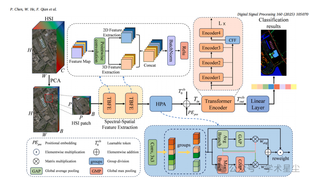
The model first reduces the spectral dimension of HSI using PCA, then utilizes the Two-Branch Feature Extraction module (TBFE) to extract spectral and spatial features in parallel. After the Hybrid Pooling Attention (HPA) module fuses cross-spatial dimension information, it inputs the data into multiple layers of Transformer encoders for global modeling, and reduces information loss through Cross-Layer Feature Fusion (CFF). Finally, a fully connected layer completes pixel-level classification, achieving efficient synergy between CNN’s local perception and Transformer’s global dependency.

1. Data Preprocessing: Utilizing PCA for dimensionality reduction, reducing spectral redundancy while preserving principal components.

2. Two-Branch Feature Extraction (TBFE): Input HSI patch, after dimensionality reduction via 1×1 convolution, is split into two branches:

   3D convolution branch: Extracts spectral correlation

   2D convolution branch: Extracts spatial texture features

   Finally, the two branches of features are concatenated

3. Hybrid Pooling Attention (HPA): Groups the concatenated features, applying average pooling and max pooling for horizontal/vertical global pooling, fusing detail and global information to achieve cross-spatial dimension attention weighting.

4. Transformer Encoder: Multi-head self-attention + MLP structure, capturing high-level spectral-spatial dependencies.

5. Cross-Layer Feature Fusion (CFF): Weighted fusion of outputs from multiple encoder layers, inputting into the final encoding layer to reduce information loss.

6. Classification Layer: Fully connected layer outputs the category of each pixel.

Main Applicable Scenarios

1. Audio and Video Processing

   Noise reduction, echo cancellation, reverb suppression

   Audio enhancement, equalization

   Video image filtering, stabilization, anti-shake

2. Communication Signal Processing

   Modulation/Demodulation

   Encoding/Decoding (e.g., audio/video codec, wireless communication protocol processing)

   Channel equalization, bit error rate optimization

3. Radar, Sonar, Medical Imaging

   Signal filtering, feature extraction

   Pulse compression, beamforming

4. Sensor Data Processing (IoT/Industrial Inspection)

   Noise reduction, feature computation, frequency domain analysis

   Preprocessing before model inference

5. Hyperspectral/Remote Sensing Images

• Band selection, spectral feature extraction

• Dimensionality reduction (e.g., PCA), noise suppression

2. Role in the System

1. Accelerate Computation: Executes FFT, convolution, filtering, etc., faster than general CPUs through dedicated hardware or optimized algorithms.

2. Reduce Main Processor Load: The DSP module handles heavy signal processing, allowing the main CPU to focus on control logic and higher-level tasks.

3. Lower Latency: Especially in real-time communication, audio/video live streaming, and industrial control, DSP can complete processing within milliseconds.

4. Modular Expansion: As a plug-and-play module, it can be flexibly replaced according to needs (e.g., different algorithm firmware), quickly adapting to different signal processing tasks.

5. Improve Processing Accuracy: Custom algorithm optimization tailored to signal characteristics enhances signal-to-noise ratio and result quality.

Summary in One Sentence

In plug-and-play systems, the DSP module is primarily used in scenarios requiring high-speed, low-latency, and high-precision signal processing, playing a role in accelerated computation, real-time processing, and reducing the main processor load.

import torch
from torch import nn
# Hybrid pooling attention (HPA)
class HPA(nn.Module):
    def __init__(self, channels, c2=None, factor=32):
        super(HPA, self).__init__()
        self.groups = factor
        assert channels // self.groups > 0
        self.softmax = nn.Softmax(-1)
        self.agp = nn.AdaptiveAvgPool2d((1, 1))
        self.map = nn.AdaptiveMaxPool2d((1, 1))
        self.pool_h = nn.AdaptiveAvgPool2d((None, 1)) #Y avg
        self.pool_w = nn.AdaptiveAvgPool2d((1, None)) #X avg
        self.max_h = nn.AdaptiveMaxPool2d((None, 1)) #Y avg
        self.max_w = nn.AdaptiveMaxPool2d((1, None)) #X avg

        self.gn = nn.GroupNorm(channels // self.groups, channels // self.groups)
        self.conv1x1 = nn.Conv2d(channels // self.groups, channels // self.groups, kernel_size=1, stride=1, padding=0)
        self.conv3x3 = nn.Conv2d(channels // self.groups, channels // self.groups, kernel_size=3, stride=1, padding=1)

    def forward(self, x):
        b, c, h, w = x.size()
        group_x = x.reshape(b * self.groups, -1, h, w) # b*g,c//g,h,w --->2048,2,11,11
        x_h = self.pool_h(group_x) #2048,2,11,1
        x_w = self.pool_w(group_x).permute(0, 1, 3, 2) #2048,2,1,11--->2048,2,11,1
        hw = self.conv1x1(torch.cat([x_h, x_w], dim=2)) #2048,2,22,1
        x_h, x_w = torch.split(hw, [h, w], dim=2) #2048,2,11,1
        x1 = self.gn(group_x * x_h.sigmoid() * x_w.permute(0, 1, 3, 2).sigmoid()) #2048,2,11,11
        x2 = self.conv3x3(group_x) #2048,2,11,11

        y_h = self.max_h(group_x) #2048,2,11,1
        y_w = self.max_w(group_x).permute(0, 1, 3, 2)
        yhw = self.conv1x1(torch.cat([y_h, y_w], dim=2)) #2048,2,22,1
        y_h, y_w = torch.split(yhw, [h, w], dim=2) #2048,2,11,1
        y1 = self.gn(group_x * y_h.sigmoid() * y_w.permute(0, 1, 3, 2).sigmoid()) #2048,2,11,11
        y11 = y1.reshape(b * self.groups, c // self.groups, -1) # b*g, c//g, hw 2048,2,121
        y12 = self.softmax(self.map(y1).reshape(b * self.groups, -1, 1).permute(0, 2, 1)) #2048,1,2

        x11 = x1.reshape(b * self.groups, c // self.groups, -1) # b*g, c//g, hw 2048,2,121
        x12 = self.softmax(self.agp(x1).reshape(b * self.groups, -1, 1).permute(0, 2, 1)) #2048,2,1,1-->2048,2,1--->2048,1,2
        x21 = x2.reshape(b * self.groups, c // self.groups, -1) # b*g, c//g, hw #2048,2,121
        x22 = self.softmax(self.agp(x2).reshape(b * self.groups, -1, 1).permute(0, 2, 1)) #2048,2,1,1-->2048,2,1--->2048,1,2
        weights = (torch.matmul(x12, y11) + torch.matmul(y12, x11)).reshape(b * self.groups, 1, h, w)
        return (group_x * weights.sigmoid()).reshape(b, c, h, w) 
    
if __name__ == "__main__":
    # Module parameters
    batch_size = 1    # Batch size
    channels = 32     # Number of input feature channels
    height = 256      # Image height
    width = 256        # Image width

    model = HPA(channels=channels)
    print(model)
    
    # Generate random input tensor (batch_size, channels, height, width)
    x = torch.randn(batch_size, channels, height, width)

    # Print the shape of the input tensor
    print("Input shape:", x.shape)

    # Forward propagation to compute output
    output = model(x)

    # Print the shape of the output tensor
    print("Output shape:", output.shape)

For more analysis, see the original text