Reprint with permission: Spiral – Clinical Doctor Research Growth Platform

ImageJ (Official website: https://imagej.nih.gov/ij/) is a public image processing software based on Java, developed by the National Institutes of Health (NIH). It is a powerful free software that plays a very important role in biological and medical image analysis.
The image below is the interface of the ImageJ official website. Download the corresponding software according to your system under Download. ImageJ is compatible with Mac OS X, Linux, and Windows systems (not limited by computer system). Counting is very common in biomedical fields, let’s explore counting with ImageJ together.
1
Manual Counting
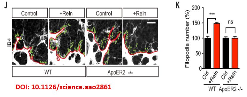
Counting with the Multi-Point Tool
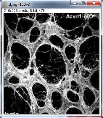
Open the ImageJ software, go to File, Open to open the image to be analyzed:
Click the  point tool, right-click, and select
  Multi-Point Tool, manually click to count:
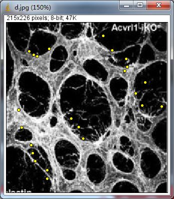
Click Analyze –> Measure, and you can see that the current count is 23. Save the image.
Cell Counter for Cell Counting
Click Plugins –> Analyze –> Cell Counter, the interface is as follows:
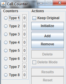
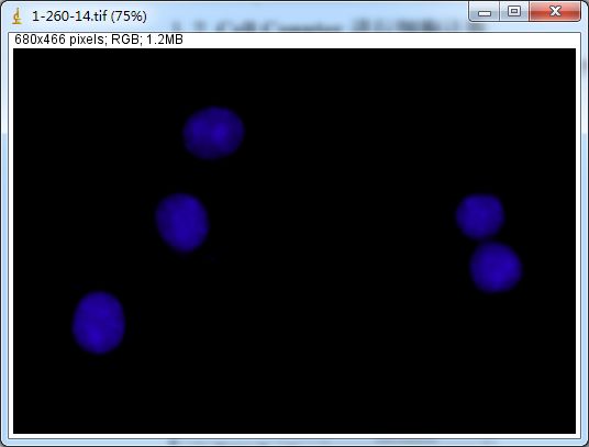
Click Initialize to count different types of cells:
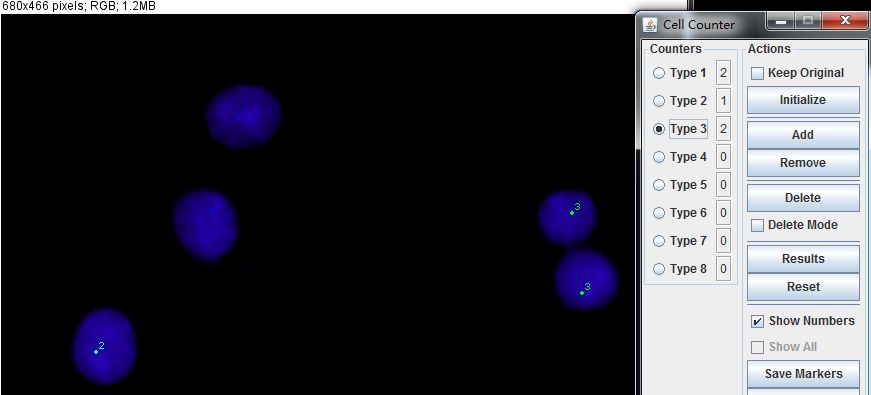
You can see that the counts for Type1, Type2, and Type3 are 2, 1, and 2 respectively. This method can count different types of cells simultaneously. Click Results in Cell Counter to see the number of different cell types. Compared to the Multi-Point manual counting method, Cell Counter can count different cell types.

2
Regular Automatic Counting Process
Open ImageJ software, go to File –> Open to open the image that needs to be analyzed:
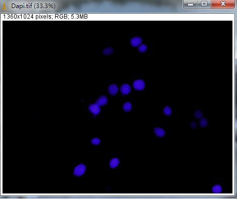
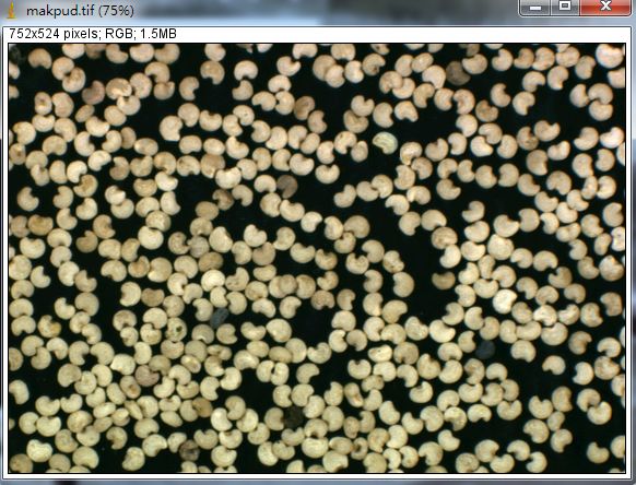
Image –> Type -> 8-bit (change to grayscale image)
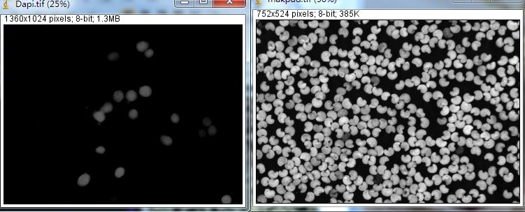
Image -> Adjust -> Threshold to adjust the threshold, red represents selected, so that all cell nuclei are selected. In the Dapi image, the threshold is 11-255 –> Apply
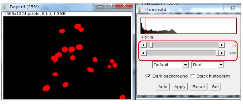
Note: The background of the fluorescence image is black, so the option below for Dark background needs to be checked, indicating that the background is black.
After Apply, the image is:
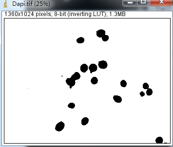
For the bean image, the threshold range is 37-255->Apply
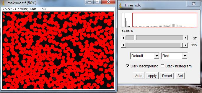
After Apply, the image is:
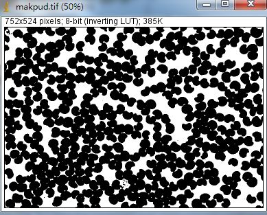
From the image after Apply, it can be seen that many cells are connected together, and during cell counting, they need to be separated.
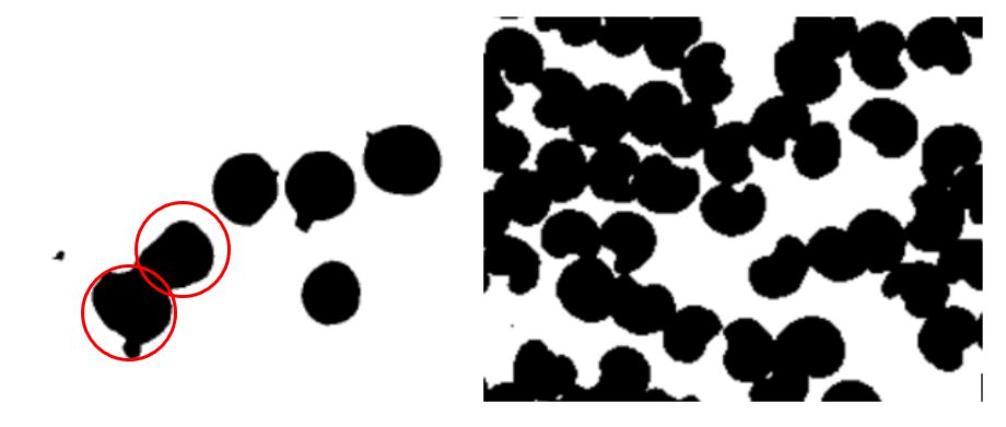
Process -> Binary -> watershed (the watershed segmentation method, separates connected cells)
The segmentation effect is as follows:
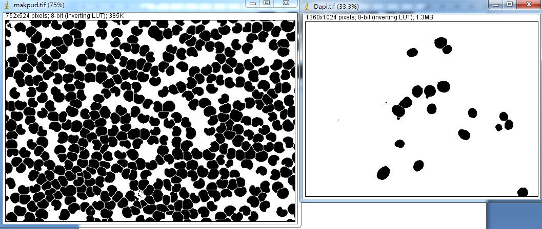
Analyze -> Analyze particles, the interface is as follows:
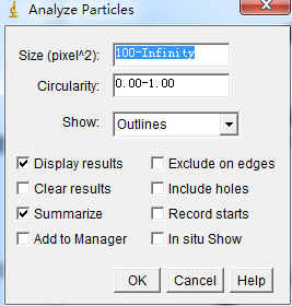
Size(pixel^2): By default 0-Infinity (infinity), meaning that the size of the cells to be counted falls within which range. For this Dapi image, the cell size is selected as 500-Infinity, filtering out non-target spots. Here we need to try a few minimum values based on the target cell size to get accurate cell counting results.
Circularity: Represents circularity, the closer to 1, the closer to circular, we do not need to change this.
Show: I habitually choose outlines to show the counted cell contours and the numbered counted cells, there are other options. Nothing means that the image and overlay will not display; Bare outlines show only the cell outlines without numbering.
Ellipses: Makes the result contours match the best elliptical shape.
Masks: Fills particles as an 8-bit black and white image.
Count Masks: Fills particle contours as a 16-bit image.
Overlay Outlines: Displays measurement particle contours in the overlay image.
Overlay Masks: Displays measurement particle contours in the overlay image, generally outlines are sufficient for cell counting.
The following option is Display results, to show results.
Clear Results:Repeated measurements of previously measured results will be cleared;
Summarize:Summarizes results;
Exclude on edges:Excludes cells touching the edges from counting;
Include holes: Internal holes will be included;
Add to Manager:Measures particles added to the ROI manager;
Record Starts:Allows plugins and macro functions to recreate particle contours;
In Situ Show:In situ display, the original image will be replaced by the binary image specified in the drop-down menu (black or white).
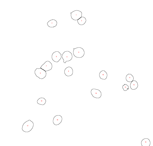
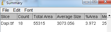
The results obtained are as follows:
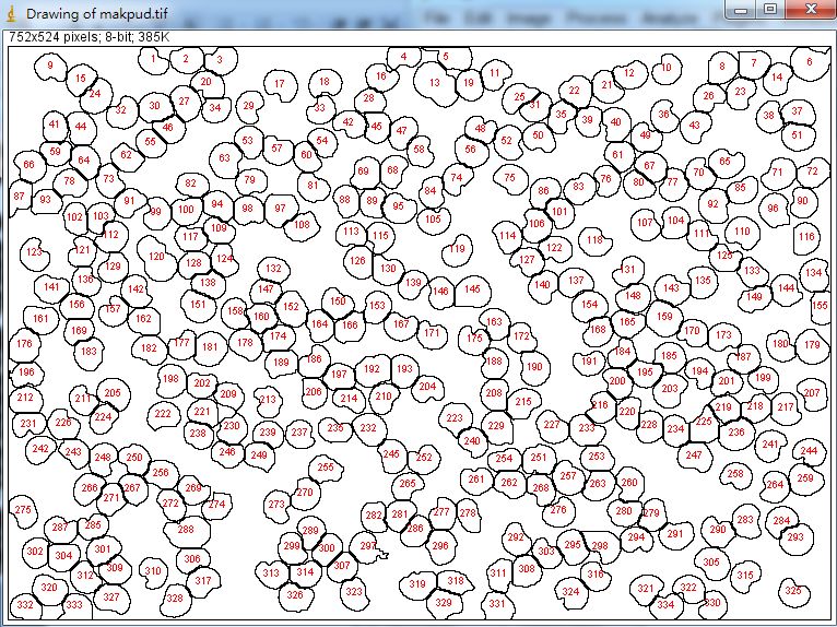
The bean results are as follows:

Application Example:
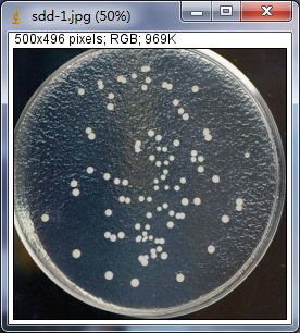
Open the image: 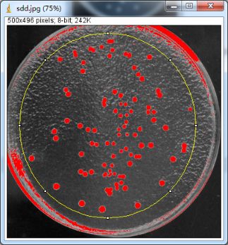
Convert RGB image to grayscale: Image –> Type –> 8-bit.
Select threshold: Image–>Adjust–>Threshold–>threshold selection–>red represents selected. The highlighted area at the edge of the dish affects the selection of colonies, use the elliptical  box to roughly select the area where the colony is located.
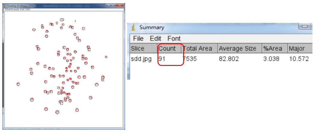
Analyze–>Analyze particles, select as follows, click OK to get the counting result:
3
Automatic Counting of Multi-Porous Materials with ImageJ
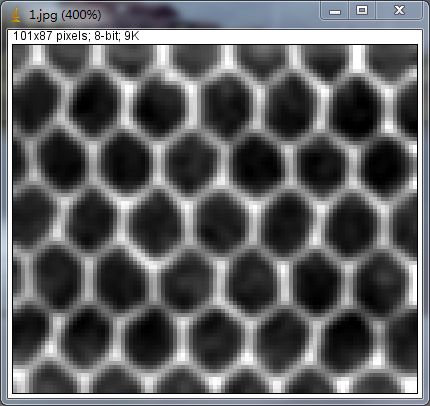
Open ImageJ software, go to File–>Open to open the image that needs to be analyzed:
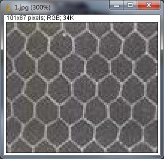
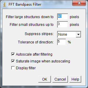
Process–>FFT–>Bandpass Filter–>OK:
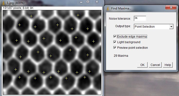
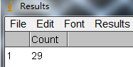
Process–>Find Maxiam–>Output type select Count to get counting data:
4
RetFM-J Automatic Counting
Open ImageJ software, go to File–>Open to open the image that needs to be analyzed:
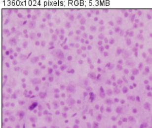
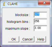
Plugins–>CLAHE Enhance Contrast–>click OK
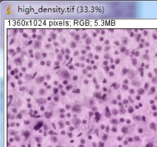
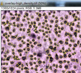
Plugins–>RetFM-J–>OK
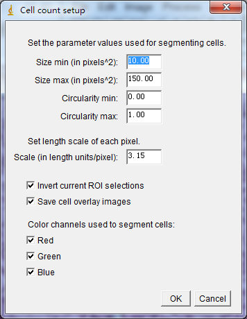
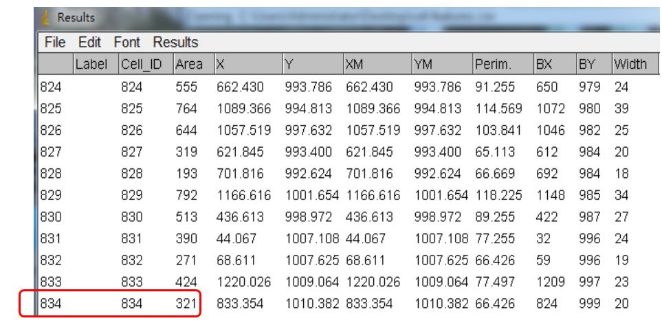
The total number of cells is 834, along with Area, coordinates (X,Y), Perim and other indicators.
5
DAB Staining for Counting
Open ImageJ software, go to File–>Open to open the image that needs to be analyzed:
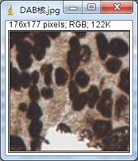
Click Plugins–>IHC tools
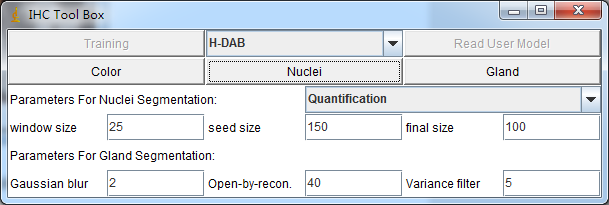
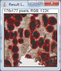
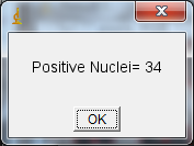
Select H-DAB–>Nuclei, the result is 34.
6
Quick Dendritic Spine Density Analysis Method and Cell Counting
Crop the dendrites to be analyzed from Golgi-stained images:
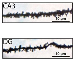
Open Fiji, go to File–>Open the dendritic spine image to be analyzed (using DG as an example)
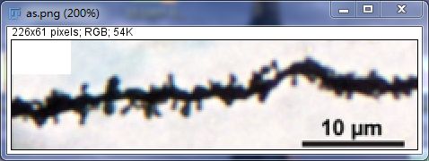
Change the image from RGB to grayscale: Image–>Type–>8-bit;
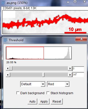
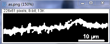
Convert the image to a binary image: Image–>Adjust–>Threshold (adjust the threshold until the dendrites and dendritic spines are fully selected), click Apply to complete binarization. The binary image is as follows (black or white, grayscale values are 0 or 255):
Calibrate the scale: click the Straight tool 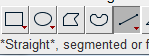 and draw a straight line on the scale while holding Shift.
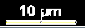
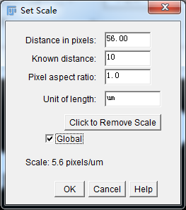
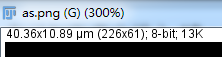
Analyze–>Set Scale–>fill in 10 μm in the known distance–>select Global so that the scale correction is valid for all images opened this time. At this point, the step 1 measurement of 226 x 61 pixels changes to 40.36 x 10.89 μm in the image below.
Skeletonizing the binarized image: Process–>Binary–>Skeletonize, to obtain the skeletonized image;
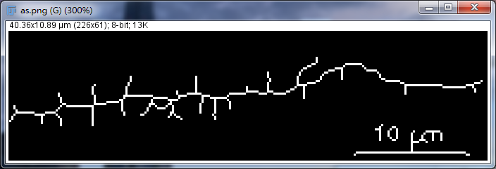
Clear the scale to avoid interference with dendritic spine counting: Select the rectangular selection in the File menu to select the scale position as shown below.
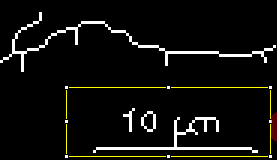
Edit–>Clear (clear the content within the selection):
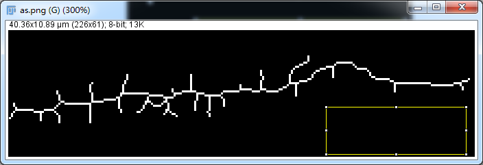
Analyze from the skeleton image to count the number of dendritic spines: Analyze–>Skeleton–>select as follows–>click OK.
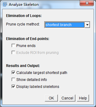
The results obtained are:
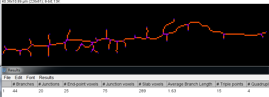
There are 25 end-point voxels, which means there are 25 dendritic spines (blue points in the image above).
The longest path to the right can be seen to be 45.31 μm (length of the dendrite), thus the spine density for this image is 25/45.31=0.55 /μm. Generally, when counting, the vertical coordinate is Spine density (Spines /10 μm), for this image it is 5.5 /10 μm.
7
Automatic Counting of Different Shapes
Open ImageJ software, go to File–>Open to open the image that needs to be analyzed, the example image contains two different shapes, 3 triangles and 4 circles:
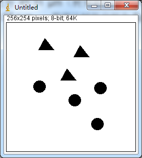
Image –> Type -> 8-bit (change to grayscale image)
Image -> Adjust -> Threshold to adjust the threshold, red represents selected, so that all shapes are selected:
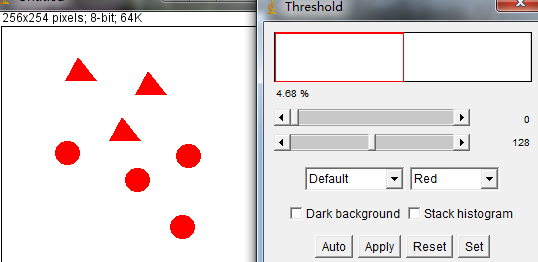
Analyze -> Analyze particles, the interface is as follows:
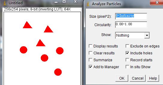
As mentioned before, Circularity represents circularity, the closer to 1, the closer to circular, we can count the two shapes based on the difference in shape circularity.
For circular shapes, set Circularity to 0.8-1, Show select Outline, and the result specifically counts 4 circular shapes:
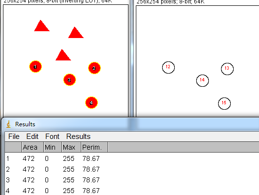
For triangular shapes, set Circularity to 0-0.5, Show select Outline, and the result specifically counts 3 triangular shapes:
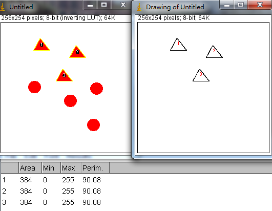
Today’s sharing on ImageJ counting ends here, hope it helps everyone. Wish you all the best in publishing articles, with the left hand CNS and the right hand, and the right hand National Natural Science Foundation!
Submission email: [email protected]