“IT Chat” is a professional information and service platform under the Machinery Industry Press, dedicated to helping readers master more professional and practical knowledge and skills in the broad field of IT, quickly enhancing workplace competitiveness. Click on the blue WeChat name to follow us quickly.
Secure Multi-Party Computation
Before discussing secure multi-party computation (hereafter referred to as MPC), we first discuss the setup of secure multi-party computation. Among all participants in MPC, some participants may be controlled by an adversary (attacker). Participants under the control of the adversary are called corrupt parties, and they will follow the adversary’s instructions to attack the protocol during execution. A secure protocol should withstand any adversary’s attack. To formally describe and prove that a protocol is “secure,” we need to precisely define the security of MPC.
1. Security
The security specification of secure multi-party computation is defined through an ideal-world/real-world paradigm. In the ideal world, there exists a trusted third party (TTP), and each participant provides their secret data to the trusted third party via a secure channel. The third party performs function computation on the joint data and returns the output to each participant. Since the only action each participant can take during the computation is to send secret data to the trusted third party, the only action the attacker can take is to choose the input of the corrupt participant, and the attacker cannot obtain any other information besides the computation result.
In contrast to the ideal world, the real world does not have a trusted third party. Participants execute the protocol without any external nodes’ help, and some participants may be “corrupted” by the attacker or collude. Therefore, a secure protocol in the real world must withstand attacks from any adversary. When the same adversary attacks in the ideal world, the joint distribution of inputs/outputs for the adversary and honest participants in the ideal world should be computationally indistinguishable from the joint distribution of inputs/outputs in the real-world execution, that is, the protocol execution in the ideal world simulates that in the real world.
The ideal-world/real-world paradigm ensures that several properties implied by “security” are satisfied.
1) Privacy: No party should gain more output than it is supposed to, especially no party should gain input information from other cooperating parties through the output. If the attacker cannot obtain any information other than the output of the corrupted party in the ideal world, then the same holds true in the real world.
2) Correctness: Every party must receive the correct output. The output received by honest participants in the real world must match the output obtained from the trusted third party in the ideal world.
3) Input Independence: The input chosen by the corrupted participant must be independent of the input from honest participants. In the ideal world, when the corrupted participant sends input to the trusted third party, it cannot obtain any input information from honest participants.
4) Output Guarantee: The corrupted participant should not have the ability to prevent honest participants from obtaining the output.
5) Fairness: The corrupted participant can only obtain the output if and only if the honest participants obtain the output, meaning there is no situation where a corrupted participant obtains the output while the honest participants do not. In the ideal world, the trusted third party always returns the output to all participants. Therefore, output and fairness can be guaranteed. This also means that in the real world, honest participants receive the same output as in the ideal world.
We need to define the participants in MPC: participants in MPC refer to all parties involved in the protocol, and each participant can be abstracted as an interactive Turing machine with a probabilistic polynomial-time algorithm (PPT Algorithm). According to the adversary’s control ability/rights over the participants during the protocol execution, the corrupted participants can be classified into three types of adversaries.
1) Semi-Honest Adversary: This type of participant executes each step according to the protocol’s requirements. However, the semi-honest adversary will try to obtain all information during the protocol execution (including execution scripts and all received messages) and attempt to infer additional privacy information.
2) Malicious Adversary: This type of participant executes the protocol entirely according to the attacker’s instructions. They will leak all inputs, outputs, and intermediate results to the attacker and may alter input information, forge intermediate and output information, or even terminate the protocol based on the attacker’s intent.
3) Covert Adversary: This type of adversary may launch malicious attacks on the protocol. Once they initiate an attack, there is a certain probability they will be detected. If they are not detected, they may have successfully completed an attack (initiating an attack to gain additional information).
Thus, based on the different attack behaviors of participants in secure multi-party computation protocols in the real world, the security model of the protocol can be classified as follows.
1) Semi-Honest Model: In this model, during protocol execution, participants follow the protocol’s specified process but may be monitored by malicious attackers who can obtain their own inputs, outputs, and information acquired during the protocol execution.
2) Malicious Model: In this model, attackers can leverage participants under their control to analyze the privacy information of honest participants through illegitimate inputs or maliciously tampering with inputs, and can also cause the protocol to terminate by preemptively terminating or refusing to participate.
Moreover, based on when and how the adversary controls participants, the adversary’s corruption strategy can be classified into the following three models.
1) Static Corruption Model: In this model, a fixed group of collaborators is controlled by the adversary before the protocol begins. Honest collaborators remain honest, while corrupted collaborators remain corrupted.
2) Adaptive Corruption Model: The adversary can decide when to corrupt which participant. It is important to note that once a participant is corrupted, they will remain in a corrupted state.
3) Proactive Security Model: Honest participants may be corrupted for a certain period, and corrupted participants may also become honest at some point. The proactive security model is discussed from the perspective of an external adversary that may invade networks, services, or devices. When the network is repaired, the adversary loses control over the machines, and the corrupted participants become honest.
In the real world, MPC protocols do not operate in isolation; they are usually combined in a modular serialized fashion or run in parallel with other protocols to form a larger protocol.
Research has shown that if an MPC protocol runs sequentially within a larger protocol, it still adheres to the real/ideal world paradigm, meaning there exists a trusted third party executing the protocol and returning the corresponding results. This theory is known as “modular composition,” which allows the construction of larger protocols using secure sub-protocols in a modular way and analyzing a larger system that uses MPC for certain computations.
In the case of parallel running protocols, if the current protocol does not require any messages to be sent from other parallel protocols, this assumption is termed the independent setting of the protocol, which is also the fundamental security definition of MPC. In the independent setting, a parallel-running protocol behaves similarly to that executed by a trusted third party.
Finally, in some other scenarios, MPC protocols may run in parallel with other instances of the protocol, other MPC protocols, or even other insecure protocols. When protocol instances require interaction with other instances, the execution of the protocol may be insecure. The protocol in the ideal world does not include interactions with other protocols (functional functions), while in the real world, it needs to interact with another functional function, resulting in different execution conditions from the ideal world simulation (the real world at this time can be termed a mixed world). In this case, the mainstream approach is to adopt “Universal Composability” for security definition, under which any protocol proven to be secure is guaranteed to execute according to ideal behavior, regardless of whether it runs in parallel with any other protocol.
The security definition of MPC plays an important role. Specifically, if an MPC protocol is secure in the real world, then for a practitioner using the MPC protocol, they can only consider the execution of the MPC protocol in the ideal world, that is, for non-cryptographic users of the MPC protocol, they do not need to consider how the MPC protocol operates or whether it is secure, because the ideal model provides a clearer and simpler abstraction of the functionality of MPC.
Although the ideal model provides a simple abstraction, in some cases, the following issues may arise.
1) In the real world, adversaries may input any value, and the MPC protocol does not have a universal solution to prevent this situation. For example, in the “Millionaire” problem, adversaries can arbitrarily input the wealth of the corrupted participant (for instance, directly inputting the maximum value), making the adversary’s corrupted party always the “winner.” If an MPC protocol’s application relies on the correct input from participants, it is necessary to enhance/verify the correctness of participants’ inputs through other techniques.
2) The MPC protocol only guarantees the security of the computation process and cannot guarantee the security of the output. The output results of the MPC protocol may reveal the input information of other participants once all participants reveal their outputs. For instance, if two participants want to calculate their average salaries, the MPC protocol can ensure that no information other than the average salary is output. However, one participant can fully calculate the other participant’s salary based on their own salary and the average salary. Therefore, using MPC does not mean that all information can be protected.
In practice, considering the computational and communication overhead of MPC, the semi-honest model is usually the primary security setting. Therefore, the MPC protocols discussed in this book primarily focus on the semi-honest model, although some MPC protocols can support both semi-honest and malicious security, this article mainly focuses on the semi-honest setting of MPC protocols.
Cryptography
Cryptography is an important foundation of privacy computing technology and is frequently used in various technical routes of privacy computing. The theoretical system of cryptography is vast and complex. Interested readers can refer to books such as “Modern Cryptography and Its Applications” for further learning. This article will only provide a brief introduction to the basic knowledge of cryptography and commonly used cryptographic primitives in privacy computing.
In MPC protocols, two types of data encryption methods are often used: symmetric encryption and asymmetric (public key) encryption.
1) Symmetric encryption is an early application of encryption algorithms with mature technology. Since the same key is used for both encryption and decryption, it is called symmetric encryption. Common symmetric encryption algorithms include DES, AES, IDEA, etc.
2) Asymmetric encryption, also known as public key encryption, differs from symmetric encryption in that asymmetric encryption algorithms require two keys: a public key and a private key, which appear in pairs. The private key is kept secret and must not be leaked. The public key is a public key that anyone can obtain. Typically, the public key is used to encrypt data, and the private key is used to decrypt. Asymmetric encryption also has another use, which is digital signatures, where the private key is used to sign data, and the public key is used to verify the signature. Digital signatures allow the public key holder to verify the identity of the private key holder and prevent the content published by the private key holder from being tampered with. Common asymmetric encryption algorithms include RSA, EIGamal, D-H, ECC, etc.
1. Elliptic Curve Cryptography
Elliptic curve cryptography is a type of public key encryption technology, often combined with other public key encryption algorithms to obtain corresponding elliptic curve version encryption algorithms. It is generally believed that elliptic curves can achieve higher security with shorter keys.
Elliptic curve cryptography constrains the additive group of elliptic curves over the real number domain to a prime field, constructing encryption algorithms based on the difficulty of the discrete logarithm problem. An elliptic curve over the real number domain is typically defined by a binary cubic equation. For example, using the commonly used Weierstrass elliptic curve equation:

Where, a and b are configurable parameters. The set of all solutions (all points on the curve corresponding to the equation in the two-dimensional plane) plus a point at infinity, denoted as 0 (the identity element of the group, the point 0), constitutes the set of elements of the elliptic curve. On this set of points, corresponding addition and inverse operations satisfying closure, commutativity, and associativity can be defined to form the elliptic curve additive group. By modifying different parameters a and b of the elliptic curve, different elliptic curve groups can be obtained, as shown in Figure 1.

Figure 1. Elliptic curve groups with different parameters
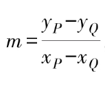
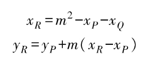
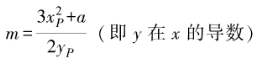
For two points P and Q on the elliptic curve, we first define the line passing through the two points and the intersection point R with the elliptic curve. The addition result of P and Q on the elliptic curve is the symmetric point of R with respect to the x-axis. This addition operation definition includes various cases, as shown in Figure 2.
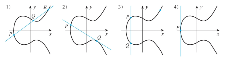
Figure 2. Four different point addition cases on the elliptic curve
1) If P and Q are not intersection points and are not inverses of each other, there is a third intersection point R, in which case P + Q = -R.
2) If P or Q is an intersection point (let’s assume 0), the line connecting P and 0 is called the tangent line. In this case, R = O, so P + Q + Q = 0. That is, the addition result is P + O = -Q.
3) If the line connecting P and Q is vertical to the x-axis, and there are no intersection points with the elliptic curve, it is considered that the intersection point is at infinity, thus P + Q = 0.
4) If P = Q, then the line is considered the tangent line of the elliptic curve at point P. If this tangent line intersects the elliptic curve at point R, the result is -R; otherwise, the intersection point is considered the point at infinity.
In terms of implementation, elliptic curve addition first calculates the slope of the line connecting P and Q.
Then, using Viète’s theorem, the coordinates of the intersection point R are calculated:
If P and Q are the same point, the slope calculation is modified to:
Then, the coordinates of R are calculated according to the above formula.
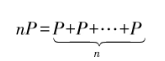
The scalar multiplication of points on the elliptic curve (also known as point multiplication) can be achieved through repeated addition of points, such as nP representing the addition of n points of P:
Since the elliptic curve additive group satisfies the commutative and associative properties, it can be optimized using the Double-and-Add algorithm.
When applying the elliptic curve additive group to encryption, it is usually required to constrain the elements of the elliptic curve to a prime field. Thus, based on its scalar multiplication, the discrete logarithm problem can be constructed. The definition of an elliptic curve over a prime field is as follows:
 a=-1, b=3 is an example of an elliptic curve point distribution over a prime field, as shown in Figure 3.
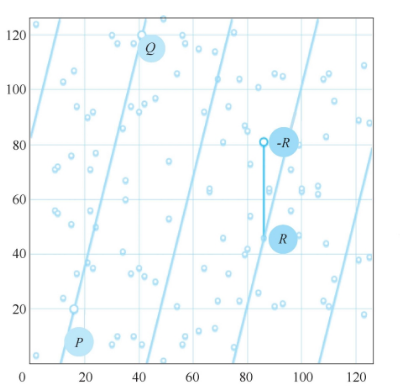
Figure 3
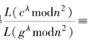
For points defined on the prime field , the addition and scalar multiplication of coordinates on the elliptic curve follow the same rules as calculations in the real number domain, but all calculations must be performed in the prime field E. As shown in Figures 1-3, the intersection point of point P (16,20) and point 0 (41.120) is point R (86,46) on the line defined under the prime field [where the line defined under the prime field includes all points satisfying ax + by + c ≡ 0 (mod p). The addition result is -R(86,81).
Similarly, based on the addition calculation rules, the scalar multiplication in the prime field can be obtained. When the scalar n is large, after calculating Q = nP, point Q can be used as the public key, and n as the private key. Knowing P and Q allows the construction of the discrete logarithm problem of the elliptic curve over the prime field. Clearly, if n is defined in the integer domain, the set of points obtained from the scalar multiplication of P constitutes the cyclic subgroup of the elliptic curve. To ensure security, it is necessary to have enough points covered by the scalar multiplication of P (the order of the subgroup must be sufficiently large), so a base point with a higher order of elements should be found.
A simple method to find the base point is to first determine the order N of the elliptic curve and the order n of the subgroup (which needs to be a prime), calculate the cofactor h = N/n, and then randomly select a point P in the elliptic curve, compute G = hP. If G = 0, select the point again; otherwise, point G will be the base point.
There are multiple mainstream elliptic curves and parameters considered secure, such as the elliptic curve secp256k1 used in Bitcoin signatures, curve25519, etc.; the open-source framework FATE implements the twisted Edwards curve Edwards25519.
, the addition and scalar multiplication of coordinates on the elliptic curve follow the same rules as calculations in the real number domain, but all calculations must be performed in the prime field E. As shown in Figures 1-3, the intersection point of point P (16,20) and point 0 (41.120) is point R (86,46) on the line defined under the prime field [where the line defined under the prime field includes all points satisfying ax + by + c ≡ 0 (mod p). The addition result is -R(86,81).
Similarly, based on the addition calculation rules, the scalar multiplication in the prime field can be obtained. When the scalar n is large, after calculating Q = nP, point Q can be used as the public key, and n as the private key. Knowing P and Q allows the construction of the discrete logarithm problem of the elliptic curve over the prime field. Clearly, if n is defined in the integer domain, the set of points obtained from the scalar multiplication of P constitutes the cyclic subgroup of the elliptic curve. To ensure security, it is necessary to have enough points covered by the scalar multiplication of P (the order of the subgroup must be sufficiently large), so a base point with a higher order of elements should be found.
A simple method to find the base point is to first determine the order N of the elliptic curve and the order n of the subgroup (which needs to be a prime), calculate the cofactor h = N/n, and then randomly select a point P in the elliptic curve, compute G = hP. If G = 0, select the point again; otherwise, point G will be the base point.
There are multiple mainstream elliptic curves and parameters considered secure, such as the elliptic curve secp256k1 used in Bitcoin signatures, curve25519, etc.; the open-source framework FATE implements the twisted Edwards curve Edwards25519.
Homomorphic Encryption
If the encrypted ciphertext can be directly computed, the corresponding encryption technology is referred to as homomorphic encryption. The concept of “homomorphic” comes from the homomorphic mapping in abstract algebra, which refers to a class of mappings between two algebraic systems (groups/rings/fields) that can preserve operations, meaning for algebraic systems if through a certain mapping
 after
after F(A·B) = F(A)XF(B), it can be said that F is a homomorphic mapping from A to B.
If a plaintext is encrypted by a certain encryption algorithm, and the ciphertext undergoes a “corresponding” operation with the plaintext, the decryption yields a result that is the same as the operation performed on the plaintext, then this encryption algorithm is considered to have homomorphic properties, allowing for homomorphic encryption of the plaintext. Homomorphic encryption can be classified into three types based on the types of computations supported and their extent: Partially Homomorphic Encryption (PHE), Somewhat Homomorphic Encryption (SWHE), and Fully Homomorphic Encryption (FHE).
(1) Partially Homomorphic Encryption
F(A·B) = F(A)XF(B), it can be said that F is a homomorphic mapping from A to B.
If a plaintext is encrypted by a certain encryption algorithm, and the ciphertext undergoes a “corresponding” operation with the plaintext, the decryption yields a result that is the same as the operation performed on the plaintext, then this encryption algorithm is considered to have homomorphic properties, allowing for homomorphic encryption of the plaintext. Homomorphic encryption can be classified into three types based on the types of computations supported and their extent: Partially Homomorphic Encryption (PHE), Somewhat Homomorphic Encryption (SWHE), and Fully Homomorphic Encryption (FHE).
(1) Partially Homomorphic Encryption
Partially homomorphic encryption refers to encryption algorithms that support only addition or multiplication operations, which can be referred to as additive homomorphism and multiplicative homomorphism, respectively. Common partially homomorphic encryption algorithms include RSA, EIGamal, ECC-EIGamal, and Paillier, among which RSA and EIGamal have multiplicative homomorphic properties, while ECC-EIGamal and Paillier have additive homomorphic properties. Paillier is a commonly used partially homomorphic encryption algorithm. It is constructed based on the difficulty of the composite residue class problem and has been proven to be very reliable after years of research, and is frequently used in various open-source privacy computing frameworks. Below is a brief introduction to the principles of Paillier.
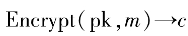
A PHE typically includes the following functionalities.
1) KeyGen(): Key generation, used to produce the public key pk and private key sk for encrypting data, as well as some public parameters (public parameter).
2) Encrypt(): The encryption algorithm, which uses pk to encrypt user data m, obtaining ciphertext (ciphertext) c.
3) Decrypt(): The decryption algorithm, which uses sk to decrypt ciphertext c, obtaining the original data (plaintext) m.
4) Add(): Homomorphic addition of ciphertext, inputting two ciphertexts c1 and c2, performing homomorphic addition.
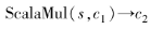
5) ScalaMul(): Homomorphic scalar multiplication of ciphertext, inputting c and a scalar s, calculating the result of c multiplied by the scalar.
For Paillier encryption, the implementation of each algorithm function is as follows.
1) KeyGen(). Randomly generate two independent large prime numbers p and q, satisfying gcd(pg,(p-1)(q-1))=1, and p and q have equal lengths. Calculate n=pq, A=lcm(p-1,q-1), =
= (n) is the Carmichael function of n, and Icm is the least common multiple. Randomly choose
 and set g=n+1, and define the L function
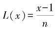 and
and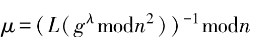 . Return public key (n,g) and private key (
 ,
, ).
).
2) . Input plaintext message m, randomly select
 to calculate ciphertext
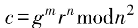
3)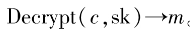 . Input ciphertext message c, calculate
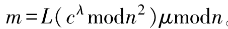 . The correctness of decryption can be verified based on the properties of the Carmichael function,
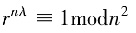 and the binomial theorem (1+x)”=1+
 to derive and verify.
From we can derive
 .
.
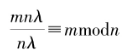
4) . Input ciphertext
 , its ciphertext addition is defined as
 Correctness can be verified:.
5) . Input ciphertext c and scalar s, its scalar multiplication is defined as
Correctness can be verified:.
(2) Somewhat Homomorphic Encryption
Somewhat homomorphic encryption (limited homomorphic encryption) supports both ciphertext addition and multiplication, but it often only supports a limited number of ciphertext multiplications. Somewhat homomorphic encryption serves as the basis for most fully homomorphic encryption schemes. Fully homomorphic encryption algorithms often add bootstrapping or progressive modulus switching to somewhat homomorphic encryption schemes. The fully homomorphic encryption algorithm originated from Gentry’s proposal in 2009, which controls the growth of noise during operations by incorporating bootstrapping into the somewhat homomorphic encryption algorithm. The bootstrapping method involves transforming the decryption process itself into a homomorphic operation circuit and generating new public and private key pairs, encrypting the original private key and the original ciphertext containing noise, and then using the ciphertext of the original private key to perform homomorphic operations on the original ciphertext, resulting in a new ciphertext without noise.
(3) Fully Homomorphic Encryption
In 2009, Gentry proposed a fully homomorphic encryption algorithm based on the circuit model, which supports both addition and multiplication homomorphic operations (Boolean operations) for each bit. Currently, mainstream homomorphic encryption schemes are constructed based on the Learning With Errors (LWE) / Ring-LWE (RLWE) problem on lattices. Both LWE and RLWE can be reduced to hard problems based on lattices, such as the Shortest Independent Vector Problem (SIVP). However, the LWE problem involves matrix and vector multiplication, making the calculations more complex, while the RLWE problem only involves polynomial operations over rings, resulting in lower computational overhead. Therefore, although mainstream homomorphic encryption algorithms (such as BGV, BFV, etc.) can be constructed based on both LWE and RLWE, RLWE is primarily used in implementations. Additionally, in 2017, Cheon et al. proposed a fully homomorphic encryption scheme for floating-point numbers—CKKS, which supports homomorphic operations for floating-point addition and multiplication for real or complex numbers, yielding approximate results. It is generally suitable for scenarios such as training machine learning models that do not require precise results.
3. Pseudo-Random Functions
Another widely used cryptographic primitive in privacy computing is the pseudo-random function (PRF). A pseudo-random function is a deterministic function of the form y = F(k,x), where k is a key from the key space K, x is an element from the input space X, and y is an element from the output space Y. Its security requirement is: given a random key k, the function F(k,·) should appear like a random function defined from X to Y. Oded et al. have proven that pseudo-random functions can be constructed using pseudo-random number generators.
Machine Learning
From the perspective of privacy computing based on its protected computation process, a large category is privacy-preserving machine learning. Machine learning can generally be divided into three types based on its learning method: supervised learning, semi-supervised learning, and unsupervised learning.
Supervised learning is a learning method given labeled training data, aiming to learn a model (function) from the provided training dataset, which can give prediction results when new data appears. Common supervised learning algorithms include Naive Bayes, Logistic Regression, Linear Regression, Decision Trees, Ensemble Trees, Support Vector Machines, (Deep) Neural Networks, etc. However, in many practical problems, the cost of labeling data is often high, so usually only a small amount of labeled data and a large amount of unlabeled data can be obtained. Semi-supervised learning is a learning method given a small amount of labeled training data and a large amount of unlabeled data. It uses unlabeled data to gain more information about the data structure, aiming to achieve better results than supervised learning techniques trained solely on labeled data. Common semi-supervised learning strategies include self-training, PU Learning, Co-training, etc. Common tasks in unsupervised learning include clustering, representation learning, and density estimation. These tasks aim to understand the intrinsic structure of the data without explicitly provided labels. Common unsupervised learning algorithms include k-means clustering, Principal Component Analysis, and Autoencoders, etc. Due to the lack of labels, most unsupervised learning algorithms do not have specific methods for comparing model performance.
In practical applications, supervised learning has a wider range of applications, so this article primarily introduces some basic concepts of supervised learning.
1. Loss Function
Supervised learning typically provides labeled training data (x,y), where x represents the input data, usually represented by a vector, with each element termed a feature; y is the output data that the model needs to learn, commonly referred to as the label. Training data generally consists of multiple (x,y) data pairs, with each (x,y) data pair termed a sample. The input of all samples constitutes the input space/feature space X, while all output labels constitute the output space Y. Based on the distribution of the output space, supervised learning can be divided into classification models and regression models. Classification models are usually divided into binary classification models and multi-class classification models based on the cardinality of the output label y.
Thus, the goal of supervised learning is to find a model f(x,w) through a learning algorithm on the training set X×Y so that the model obtains prediction values
 that are consistent with the true output values. However, the model’s predicted values
 may or may not be consistent with y. Therefore, it is necessary to use a loss function to quantify the difference between the model’s predicted values
 and the true value y (commonly referred to as the residual -y). The loss function L(y,f(x,w)) is a non-negative real-valued function that needs to be defined differently based on the task type of supervised learning. Common loss functions include 0-1 loss function, squared loss function, logarithmic loss function, cross-entropy loss function, hinge loss function, etc. However, the aforementioned loss functions are only defined based on the expected loss on the training dataset, commonly referred to as empirical loss or empirical risk. Only when the sample size approaches infinity can the loss be considered the expected loss (commonly referred to as expected risk). When the model parameters are complex and the training data is limited, there may be a phenomenon where the model predicts correctly on the training data but performs poorly on unseen data, known as “overfitting.” To prevent overfitting, a regularization term (regularized loss) is typically added on top of the empirical loss to restrict the complexity of the model parameters, resulting in a new loss function termed the structured loss function (or structural risk function).
2. Gradient Descent
Once the loss function is defined, optimization methods can be used to find model parameters that minimize the loss value. The lower the loss value, the closer the model’s predicted values
 are to the true output values y. A common parameter optimization method is gradient descent, where for each training iteration, the gradient of the loss function with respect to the parameters (the first-order continuous partial derivative) is calculated, and the parameters are updated by multiplying the negative gradient (the negative value of the gradient) by a certain step size lr (learning rate):
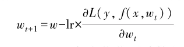
The step size lr can be fixed as a ratio or calculated adaptively through various optimizers. Gradient descent can be classified based on the selection strategy of training samples into stochastic gradient descent (selecting one sample randomly each time), batch gradient descent (using all samples each time), and mini-batch gradient descent (selecting a batch of samples sequentially each time).
In federated learning, one party with labels can directly compute the gradient. For the unlabeled party, the gradient must be computed in a secure manner, which can be achieved by having the labeled party homomorphically encrypt the residual and send it to the unlabeled party for computation, or through joint computation using MPC.
3. Deep Learning
Deep learning is a very popular machine learning method in recent years. Compared to traditional machine learning, deep learning primarily employs deep neural networks as specific model structures, optimizing various aspects such as layer structure, layer connection methods, connection weight sampling, unit structure, activation functions, learning strategies, and regularization to achieve model performance that greatly exceeds traditional machine learning. Various classic deep learning techniques are widely adopted, including Convolutional Neural Networks (CNN), Graph Convolutional Networks (GCN), Dropout, Pooling, Long Short-Term Memory Networks (LSTM), RNN, GRU, Residual Networks, DQN, DDQN, Batch Normalization, Layer Normalization, Attention, Transformer, etc.
Due to the complexity of deep learning models and the large number of parameters, and because many computations in privacy computing involve ciphertext computations, simpler neural networks with fewer layers and structures are typically used in practical applications, such as CNN, Dropout, Pooling, Batch Normalization, Layer Normalization, etc. There are various implementation solutions in privacy computing. In federated learning, the forward computation of the neural network is usually performed locally by the participants, followed by gradient computation at the coordinating node, and finally, backpropagation of the network is performed locally. Deep neural networks implemented using MPC typically involve secret sharing of model parameters and data for fully secure training or prediction. Solutions based on fully homomorphic encryption such as CKKS can perform network training and prediction directly under full encryption (data encryption or model encryption), ensuring complete separation of models and data.
The above content is excerpted from “Privacy Computing: Practical Open Source Architecture”
Recommended Reading

Click “Read the Original” for more details
Privacy computing refers to a collection of technologies that achieve data sharing, analysis, computation, and modeling while protecting the data itself from external leakage, aiming for data to be “usable but invisible.” Privacy computing involves multiple disciplines and technical systems. From the perspective of the technologies employed, it includes three main technical routes: federated learning, secure multi-party computation, and trusted execution environments.
This book mainly introduces two technical routes: federated learning and secure multi-party computation, combining theoretical knowledge with code analysis, installation, and operation based on open-source architecture. Chapter 1 introduces the basic theoretical knowledge required for privacy computing; Chapter 2 introduces federated learning modeling processes combined with the open-source framework FATE; Chapters 3-5 introduce secure multi-party computation, including oblivious transfer, secret sharing, and obfuscated circuits; Chapter 6 introduces privacy-preserving secure joint analysis, covering the SQL plan optimization and mixed execution of clear and encrypted data in two frameworks, SMCQL and Conclave. The book provides the associated open-source architecture source code, with acquisition methods found on the back cover.
This book is suitable for beginners in privacy computing and researchers who need to quickly build privacy computing products.
Expert Recommendations


Content Structure and Supporting Resources

What is the gap between you and high-paid programmers? Just this book!
Through several code snippets, a detailed explanation of Python’s single-threaded, multi-threaded, and multi-process.
30 pages of PPT to review the high-security trusted (HiTrusT) mobile terminal architecture and key technology sharing.
Author: Ji Xu
Editor: Zhang Shuqian
Reviewer: Cao Xinyu