Click to listen to music while watching☝ (Today’s recommendation: “Salon”)
FFT is an efficient algorithm for DFT, known as the Fast Fourier Transform (FFT).Fourier Transform is one of the most fundamental methods for time-domain to frequency-domain transformation analysis. TheDiscrete Fourier Transform (DFT) applied in digital processing is the foundation of many digital signal processing methods.
Due to the rapid development of computer technology, in the mid-1970s, some electronic device companies in the United States and Japan began to design and produce digital Fourier analyzers, but due to the large computational load ofDiscrete Fourier Transform, it wasn’t until the discovery of the fast algorithm (FFT) that DFT truly gained widespread application.
FFT is an efficient algorithm for DFT, known as the Fast Fourier Transform (FFT). The FFT algorithm can be divided into time-domain extraction algorithms and frequency-domain extraction algorithms, starting with a brief introduction to the basic principles of FFT. We will explain the basic principles of FFT starting from DFT operations.
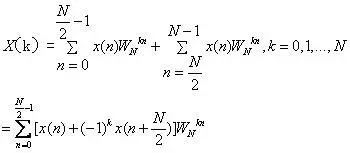
The DFT operation is:
 Figure 1
FFT can be divided into two categories: time extraction and frequency extraction, and general time extraction and frequency extraction can only handle lengths of N=2^M. Additionally, there is a combinatorial base-four FFT to handle FFT of general lengths.
The so-called extraction refers to the process of dividing a long sequence into short sequences, which can be done in either the time domain or the frequency domain. The most commonly used time-domain extraction method is to continuously transform long sequences into short sequences based on odd and even, resulting in the input sequence being in reverse order and the output sequence being in sequential arrangement, which is the Cooley-Tukey algorithm.
FFT (Fast Fourier Transform) is a super classic algorithm in digital signal processing, and most people who have studied DSP or chip design know this algorithm. However, have you ever thought about why there are so many FFTs in digital signal processing? Some might say it is to analyze the signal spectrum. Then the following question is, how does spectrum analysis relate to our daily needs, such as making phone calls, radar measuring speed and direction, etc.? Why is FFT so important? This article presents some concise examples to explain what FFT is useful for.
Let’s recall what FFT is. Before the 1970s, we mainly used analog circuits for signal processing, such as using diodes and capacitors to perform envelope detection of AM modulated signals. With the popularity of digital systems, we can use processors or digital circuits to process signals more accurately. For example, in AM detection, we can actually use a carrier to mix the signal (multiplying by a cosine function) and then perform low-pass filtering. This process can be done using digital circuit multipliers and FIR filters. FIR filters are much higher order than low-pass filters made of diodes and capacitors, so the performance is naturally better. At the same time, since digital circuits are easy to integrate into integrated circuits, we often convert the original analog signals (such as microphone audio) into digital values through analog-to-digital converters for processing.
Such systems have several issues: one is that the signal needs to be sampled, and the other is that the signal is divided into several quantization levels. Sampling means that we no longer have the original continuous signal, but a discrete set of collected sample points. Sampling a time-domain signal inevitably causes the spectrum to become periodic. If the original spectrum is limited to a finite bandwidth, then after periodic extension, as long as the period is greater than the original bandwidth, there is actually no aliasing distortion. Digital circuits limit us to binary domain calculations such as multiplication and addition, thus we have to sample the spectrum as well, leading to periodic extension in the time domain. Fortunately, if we only take a finite length, we can assume that the uncollected parts are periodically extended (because stationary systems believe that signals can be decomposed into combinations of sine and cosine functions, and sine and cosine functions can be periodically extended, so this assumption is valid), thus we obtain discrete periodic extended point sets in both the time and frequency domains.
Since it is periodically extended, the extended parts and the main value interval (the one close to 0) have repeating values, so we only keep the main value interval part. The transformation relationship from the time-domain point set to the frequency-domain point set is called the Discrete Fourier Transform (DFT). However, its computation is too complex, so Cooley and Tukey tried to simplify it, finding some inherent operational laws of this algorithm, reducing the computational load from the original square order to NlogN order. This algorithm is called the time-extraction Fast Fourier Transform, while Sanders and Tukey researched frequency extraction and also obtained a similar low-complexity algorithm. These types of algorithms are collectively referred to as Fast Fourier Transform (FFT). The computational results of FFT are completely equivalent to DFT, but the computational load is reduced. Moreover, since the energy of the time-frequency transformation remains invariant (Parseval’s theorem), the absolute values in the frequency domain are not meaningful; we only need to obtain relative values. Thus, the quantization levels in digital systems and the scaling adjustments after digital system overflow affect the FFT computation results only in terms of precision, not correctness. Therefore, FFT perfectly meets the premise that digital systems can handle, while its computational complexity is not high, thus gaining widespread application.
So, can analog systems perform similar FFT? Yes, by constructing an array of bandpass filters equal to the number of frequency points, the signal enters this bandpass filter group, and each filter only retains the corresponding frequency point with a frequency response function similar to sinc. This would yield the FFT results. However, the cost is not something that ordinary systems can bear. Therefore, in the era before the popularization of digital circuits, FFT was basically a mathematical algorithm that was not implementable.
Now we know what FFT is. It is a transformation algorithm for the discrete computation of Fourier Transform that can be digitally computed. This algorithm computes the main value interval part of the periodic extended point set in the time domain (a finite number of points) and the result is the frequency spectrum, which is also the main value interval part of the periodic extended point set. The premise for equivalence with Fourier Transform is that the sampling rate must be greater than twice the maximum frequency of the signal (high-frequency extension without aliasing), and the part outside the finite length of the time domain is assumed to be periodically extended to infinity. To satisfy the first premise, we often add a low-pass filter before signal processing (even before analog-to-digital conversion) to suppress high-frequency components. For example, in audio or communication systems within a specific frequency band, high-frequency components are meaningless, so this premise can be satisfied.
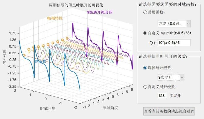
To satisfy the second premise, we need to ensure that the sampled values outside the sampling area are consistent with the values of the assumed periodic extension. This is clearly impossible, and the result of not being able to achieve this leads to what? The spectrum leakage occurs, meaning that the energy of the spectrum disperses outside the band (for example, a cosine function is no longer a single spectral line, but rather sinc). The dispersion process can be considered as the time domain being multiplied by a rectangular window (multiplied by a gate function), leading to the spectrum being equivalent to the convolution with sinc function. The smaller the time domain window (i.e., the fewer the sample points), the wider the main lobe of the spectrum sinc, and the more severe the spectrum leakage. This means that the energy of the original frequency point will be dispersed over a larger nearby range, and its peak value will decrease. If adjacent points each have peaks, then after dispersion, it becomes difficult to distinguish. Therefore, the actual resolution of the system is inversely proportional to the length of the time domain window. The more sample points we collect, the more likely we are to obtain a finer spectrum. Is there a way to reduce this leakage? The best approach is to let the values at the boundaries have less influence while giving more weight to the middle part. This effectively multiplies the sample points by a series of weighted values, forming a time-domain window function. After windowing, the spectrum leakage will be reduced, and energy will be more concentrated, but the main lobe will be wider. This is a trade-off. In this way, the two premise conditions can be approximately satisfied, although not completely, but it is sufficient.
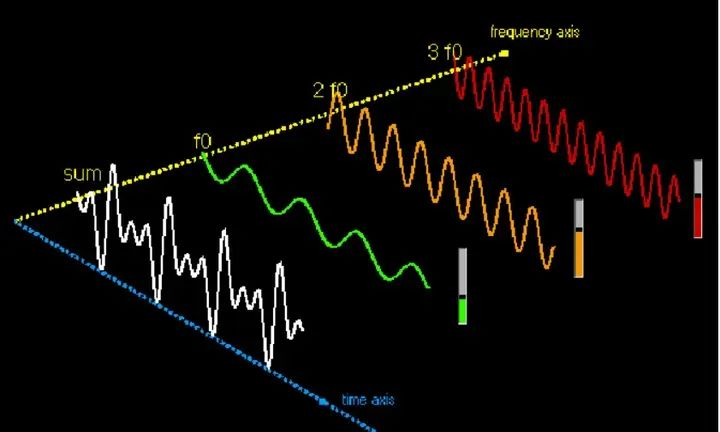
These are relatively basic concepts. Now let’s discuss some interesting matters. If FFT is only used to analyze deterministic stationary signals, such as sine waves or combinations of several sine waves in infinite long periodic signals, it would not have the status it has today. What else can it be used for?
1. Perform Fast Correlation
Correlation is extremely important in digital signal processing. Simply put, if you do not know a certain parameter in the signal (such as frequency, phase, chip sequence, or shaped waveform), you can design a group of signals that contain all possible values of this parameter and correlate them with the signal to see which result is the largest. The corresponding parameter is the most likely one. This algorithm is called maximum likelihood detection, and correlation is often the practical execution process of maximum likelihood detection. Many times, the parameter to be measured is related to time delay. For example, after a mobile phone is turned on, it needs to synchronize with the base station, meaning it needs to know the starting time of each data frame. How can this be achieved? First, the base station and the mobile phone have a protocol, and at a certain position in the frame, there will be a fixed sequence. This sequence will have a fixed waveform after modulation, so the mobile phone can create several delayed copies of the waveform and correlate them with the received waveform. The peak value corresponding to the delay can then be converted into the starting time of the frame.
We will discuss the power of correlation later, but what is the relationship between correlation and FFT? Correlation and convolution are both operations with very high complexity. Each time a correlation value is calculated for a delay, all corresponding non-zero parts of the two waveforms need to be multiplied and summed. The correlation values for all delays form a curve called the correlation function. However, once the signal is converted to the frequency domain, the process of obtaining the correlation function can be simplified to a process where a signal’s conjugate (the imaginary part is negated) is multiplied by another signal. Even with the overhead of two FFTs, the calculation is still significantly smaller (the difference between N squared and N log N), thus greatly reducing the complexity of the correlation algorithm.
Sometimes, if the input signal is too long, what can be done? It has been discovered that the correlation operation can be performed in segments. By performing correlation on each segment and then combining them, we get the result after correlation. This way, timing operations in mobile phones can be completed with a fast correlation process. Another example is how radar can locate a target’s distance. The simplest idea is to send an impulse signal and see when it returns; the time delay multiplied by the speed of light divided by 2 gives the distance. However, a waveform resembling an impulse function is very difficult to achieve for power amplifiers. Therefore, radar systems actually send out signals with a certain time length and a wide bandwidth, such as chirp or some shaped signal. Upon reception, we need to know how much this signal has been delayed, so we correlate it with a local copy of the shaped waveform. Successful correlation will yield a waveform with several peak points, and these peak points correspond to the echo time delay values of several targets, which can then be converted into positions. This process of compressing waveform energy into points is generally accomplished using FFT.
2. Fast Convolution
Similar to correlation, a major operation type in signal processing is convolution. A system can be represented by its system function, and its output is the input data convolved with the system function. For stationary random signals, the output is the input data convolved with the square of the magnitude of the system function. Convolution operations are often used for FIR filtering of signals because FIR filters do not have feedback and have no memory, allowing direct output via convolution algorithms. If the data is block data (not clock-timed stream data), using fast convolution can reduce computational load. The process is similar to fast correlation, with the difference that there is no need for conjugation when multiplying in the frequency domain. For example, if an FM radio receives several stations that are very close to each other, how can it filter out the desired station? A higher-order FIR bandpass filter can be used to select the desired station. For example, the DSP chip demodulated radio from Degen can achieve a resolution of 0.01MHz, which is one of the reasons why our digital FM radios sound better than the original analog FM radios.
3. Classic Spectrum Estimation
In real life, we cannot expect to see only deterministic infinite-length signals composed of sine and cosine waves. At the very least, such signals will also be superimposed with noise, i.e., Gaussian white noise. Therefore, the premise of Fourier transform spectrum analysis cannot be satisfied, and such time-frequency transformations lose practical significance. Alternatively, we often analyze infinite-length random signals that are stationary in the random sense (in terms of second-order statistical properties such as autocorrelation). If this premise cannot be met, at least it can be satisfied within a certain time period. Such signals are often random, but their autocorrelation and cross-correlation characteristics often contain second-order statistical information about the signals. For practical systems, we can only estimate them. A basic method for estimating the correlation function is to perform point multiplication between one signal and another signal that has been delayed and conjugated, obtaining a function based on the delay. As mentioned earlier, FFT can accomplish this.
In this analysis of random signals, there is an important theorem called the Wiener-Khintchine theorem, which proves the relationship between the autocorrelation of a signal and the power spectrum of the signal is the FFT transformation. This interesting bridge allows us to do several things, one of which is to estimate the power spectrum through FFT using the estimates of autocorrelation. A careful observer will notice that the last FFT in this process is immediately followed by an IFFT, which cancels out, thus only requiring one FFT instead of three. This power spectrum estimation method is called the periodogram power spectrum estimation, which is one of the most commonly used classic spectrum estimation methods. It is noteworthy that the power spectrum of a signal actually corresponds to the ideal value of autocorrelation, not the estimated value obtained from the received data (the above uses fast correlation to calculate the estimated value). If this estimation uses boundary points, the correlation values may be biased due to the assumption that the values outside the boundary are zero. If we only use several points in the center, it will be relatively more accurate. This method of calculating autocorrelation and selecting reliable points before performing Fourier transforms is called the autocorrelation method of power spectrum estimation.
Interestingly, the two methods can be combined. First, perform overlapping segmentation for periodogram estimation, take the average of these results, and then use IFFT to obtain the autocorrelation. After obtaining the autocorrelation, window it (similar to the effect of weighting mentioned earlier) to obtain a better autocorrelation estimate, and then use FFT to obtain the spectrum estimate. This method is considered a significantly improved classic spectrum estimation method called the Welch method. The acceptance of these methods is mainly due to the bridging effect of FFT. Otherwise, such methods would not be applicable to the system. Instruments such as spectrum analyzers can employ these classic spectrum estimation algorithms (of course, there are also frequency sweeping methods). Additionally, since the peak values of the power spectrum represent the frequencies of the signals, if this signal is the reflected echo of an object, the speed of the object can be calculated using the Doppler formula. A type of radar that uses this speed measurement mechanism is called pulse Doppler radar.
4. Modern Spectrum Estimation
To achieve more accurate spectrum estimation, some scholars believe that by constructing models and estimating parameters, better spectrum estimation can be obtained. As long as the system model is designed reasonably and the parameters to be estimated are effectively estimated, the spectrum estimation of the signal can be transformed into the spectrum of this model, thus obtaining more precise estimation results. This model-based spectrum estimation is called modern spectrum estimation. So, what is considered reasonable? It is generally believed that minimizing the Euclidean distance is more reasonable, which is the least squares criterion. Under this criterion, combined with the premise of linear systems, the interesting square expectation is transformed into the self-correlation and cross-correlation terms of the system (Wiener-Hopf equation). The estimation methods for these two terms, needless to say, must also be completed effectively using fast correlation, which is one reason why FFT still plays a role in modern spectrum estimation, AR models, MA models, and other theories. At least in terms of computation, the autocorrelation method is the simplest among known AR parameter estimation methods.
Once the model is estimated, we can also do other things, such as estimating the future trend of the signal based on the model, which is called signal prediction, or smoothing the collected signals using this model, etc. For example, how do you measure the position of an object? In modern radar, there is usually an antenna array. If the echo received from the object has an angle relative to the antenna array, different antennas will receive the echo at different times (different phases, with the amplitude basically unchanged). Thus, using the echo signals from several antennas, the angles of several target objects can be estimated. This is called Direction of Arrival (DOA) estimation, with two classic algorithms: MUSIC and ESPRIT. They are both second-order statistical signal algorithms, relying on the autocorrelation matrix as the starting point for calculations, thus FFT can serve as a fast algorithm for autocorrelation estimation.
5. Construct Orthogonal Systems
What pattern do the discrete frequency spectra obtained from FFT follow compared to the original continuous frequency spectrum? These parts can be considered as the result of a family of orthogonal sinc functions superimposed. It can also be viewed as the result of a sinc function with a main lobe width equal to the frequency spectrum interval width convolved with an accumulation function (since the time domain is the result of multiplying the original signal with a rectangular window). Here, orthogonal refers to the fact that the value of one discrete point has no relation to the value of another discrete point, and they do not affect each other. Such a system can be used to construct communication transceivers, as the orthogonality of sinc functions results in the best frequency spectrum efficiency (using bandwidth suppression to mitigate the sidelobes of each sub-band will extend the time-domain signal, leading to inter-symbol interference).
Orthogonal Frequency Division Multiplexing (OFDM) leverages the orthogonal characteristics between discrete frequency points to build a high-performance, low-complexity transceiver. Its working principle is to first place the data to be transmitted on each frequency point, typically using QAM or PSK modulation, then perform IFFT to obtain the time-domain signal for transmission. The time-domain waveform formed by these frequency point data is essentially a set of orthogonal cosine functions with frequency multiples. After the receiver receives this signal, it performs FFT to convert it back to the frequency domain (or orthogonal domain), thus estimating the symbols transmitted on each frequency point.
The cleverness of this system lies in overcoming the multipath fading of wideband wireless communication systems. From the perspective of the entire frequency band, the channel is not constant; some frequency points are enhanced while others are weakened, and there are also phase distortions. However, when divided into many orthogonal sub-channels, these channels can be viewed as flat. Through equalization, such as zero-forcing equalization, we can obtain characteristics of the sub-channels similar to impulse response, thus demodulating the value of the symbols on each sub-channel. Because the sub-channels are orthogonal and do not interfere with each other, multi-carrier communication can be achieved, allowing parallel transmission of all data, significantly increasing transmission speed. This is one of the core technologies that allow 4G mobile communication speeds to reach hundreds of megabits or even higher.
The significance of FFT may go beyond this, and there are many variants, such as two-dimensional FFT, DCT, etc., which contribute to image blurring (clarification), contouring, compression, and other aspects. This article serves merely as an introduction, aiming to help peers dedicated to researching and developing digital systems to better understand the principles and essence of the algorithms involved. The content mentioned is all foundational knowledge in signal processing, typically covered in general master’s courses. This organization is intended to provide some new insights for everyone.
Below, feel free to check the content according to your personal needs~
Time Extraction
Let N-point sequence x(n),

, group x(n) by odd and even, as shown in Figure 2:
 Figure 2
Rewrite to:
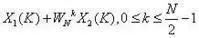 Figure 3
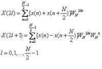
An N-point DFT is decomposed into two N/2-point DFTs,
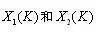 Figure 4
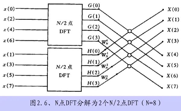
Continue to decompose,iterate down, and its computational load is approximately
 Figure 5
The algorithm has the following rules:
Two 4-point DFTs form an 8-point DFT:
 Butterfly Algorithm
Four 2-point DFTs form an 8-point DFT:
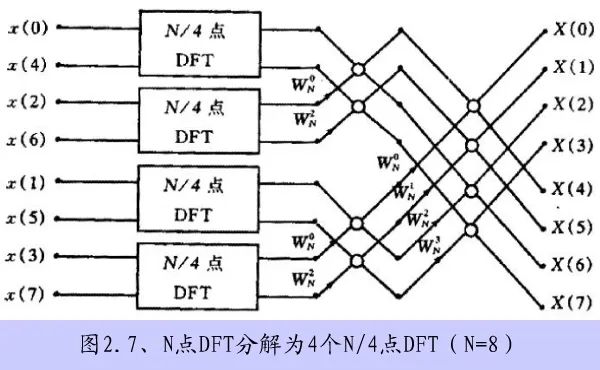
8-point DFT based on time extraction:
In-place computation
When data is input into memory, the results of each level of computation are still stored in the same set of memory until the final output, without the need for other memory.
Ordinal Reordering
For the in-place operation structure of the time extraction FFT, when the computation is completed, the storage units A(1), A(2), …, A(8) will exactly store X(0), X(1), X(2), …, X(7) in order, thus allowing direct sequential output. However, the input x(n) of this in-place computation cannot be stored in this natural order in the storage units, but must be stored in the order of X(0), X(4), X(2), X(6), …, X(7). This order seems quite chaotic, but it does have its rules. When this order is represented in binary, it exactly corresponds to the order of “bit reversal”.
The number of butterfly types increases exponentially with the number of iterations.
The number of butterfly types in each iteration doubles compared to the previous iteration, and the data point interval also doubles.
Frequency Extraction
The frequency extraction 2FFT algorithm is an algorithm that extracts based on frequency.
Let N=2^M, and decompose x(n) into two parts,
 DFT Transformation Formula
Separate into two groups based on the parity of K, that is,
 FFT Principle
Obtain two N/2-point DFT operations. Decompose this way and iterate, the total computational load is the same as the time extraction (DIT) base-2 FFT algorithm.
The algorithm rules are as follows:
The butterfly structure is different from time extraction, but the number of butterflies is the same, and it also has in-place computation rules, with the number of iterations decreasing exponentially.
Combinatorial Base-Four FFT
When N≠2^M, zero-padding can be used to make it N=2, or it can be first decomposed into two sequences p and q, where p*q=N, and then calculations can be performed.
Chirp-Z Transform
As mentioned earlier, using the FFT algorithm, one can quickly compute all N-point DFT values, that is, all uniformly spaced sample values of the z-transform X(z) on the unit circle in the z-plane. In practice, it may be the case that 1) it is not necessary to compute the entire sampling of the z-transform on the unit circle. For narrowband signals, it is sufficient to analyze a segment of the signal’s frequency band to achieve a higher resolution, while the parts outside the frequency band can be disregarded; 2) or sampling on other contours of the z-transform is of interest. For example, in speech signal processing, it is necessary to know the frequency of the poles of the z-transform. If the pole positions are far from the unit circle, the spectrum on the unit circle will be very smooth, making it difficult to identify the frequency of the poles. If sampling is not along the unit circle but along an arc close to these poles, the spectrum at the frequency of the poles will present a significant peak, allowing for a more accurate determination of the pole frequency; 3) or there is a need to effectively compute the DFT of sequences when N is prime, thus increasing the flexibility of DFT calculations.
Spiral sampling is a suitable transform for such needs and can use FFT for rapid computation. This transform is also known as the Chirp-Z transform.
FFT Calculation of IDFT
DFT transformation indicates that for time-limited signals (finite-length sequences), frequency domain sampling can also be performed without losing any information. Therefore, as long as the time sequence is long enough and the sampling is dense enough, frequency domain sampling can adequately reflect the trend of the signal’s spectrum. Thus, FFT can be used for frequency spectrum analysis of continuous signals.
Of course, several approximations have been made here:
1. Using the Fourier transform of discrete sampled signals to replace the frequency spectrum of continuous signals; the frequency spectrum will not be distorted only if the sampling theorem is strictly satisfied; otherwise, it is only an approximation; 2. Using finite-length sequences to replace infinite-length discrete sampled signals.
FFT Calculation of Linear Convolution
Linear convolution is one of the main methods for finding the response of discrete systems, and many important applications are based on this theoretical foundation, such as convolution filtering.
Previously, we discussed the method of using circular convolution to calculate linear convolution, which can be summarized as follows:
Extend the sequence x(n) of length N2 to L, padding L-N2 zeros
Extend the sequence h(n) of length N1 to L, padding L-N1 zeros
If L≥N1+N2-1, then circular convolution equals linear convolution. At this point, linear convolution can be computed using FFT as follows:
a. Calculate X(k)=FFT[x(n)]
b. Find H(k)=FFT[h(n)]
c. Find Y(k)=H(k)Y(k) for k=0 to L-1
d. Find y(n)=IFFT[Y(k)] for n=0 to L-1
It can be seen that only two FFTs and one IFFT are needed to complete the calculation of linear convolution. Calculations show that when L>32, the method of calculating linear convolution mentioned above has significant advantages over direct calculation of linear convolution, thus this circular convolution method is also referred to as fast convolution method.
FFT Calculation of Correlation Functions
Cross-correlation and autocorrelation functions can be calculated using FFT. Since discrete Fourier transform implies periodicity, using FFT to calculate discrete correlation functions is also for periodic sequences. Performing N-point FFT directly corresponds to performing periodic extension on two N-point sequences x(n) and y(n), correlating them, and then taking the main value (similar to circular convolution). However, in reality, linear correlation of two finite-length sequences is generally required. To avoid confusion, it is necessary to use a method similar to that of calculating linear convolution through circular convolution, first extending the sequences and padding zeros, then using the above method.
Real Sequence FFT
Signals are real sequences, and any real number can be considered as a complex number with zero imaginary part. For example, to find the complex spectrum of a real signal y(n), it can be viewed as adding a zero imaginary part to the real signal, transforming it into a complex signal (x(n)+j0), and then using FFT to find its discrete Fourier transform. This approach is inefficient since converting real sequences to complex sequences doubles the memory requirement, and during computer operation, even if the imaginary part is zero, operations involving the imaginary part still occur, wasting computational resources. A reasonable solution is to utilize complex data FFT for effective computation of real data. The method is described below.
An N-point FFT simultaneously computes the DFT of two independent N-point real sequences x1(n) and x2(n), where X1(k)=DFT[x1(n)] and X2(k)=DFT[x2(n)].
By treating x1(n) and x2(n) as the real and imaginary parts of a complex sequence, let
x(n)=x1(n)+jx2(n)
Through FFT computation, we can obtain the DFT value of x(n) as X(k)=DFT[x1(n)]+jDFT[x2(n)]=X1(k)+jX2(k).
Using the conjugate symmetry of discrete Fourier transform, we find:
X1(K)=1/2*[X(k)+[X(N-k) conjugate]]
X2(K)=1/2*[X(k)-[X(N-k) conjugate]]
With the FFT results of x(n), we can derive the values of X1(k) and X2(k) from the above formulas.
Note: The views expressed in this article solely represent the author’s perspective, and no guarantees or commitments are made regarding the content. Readers are advised to refer to it for reference and verify its authenticity and legality at their own discretion. If you find any errors in the attribution of images, text, or video content or if your rights are infringed, please inform this public account, and we will promptly make modifications or deletions.