Skip to content
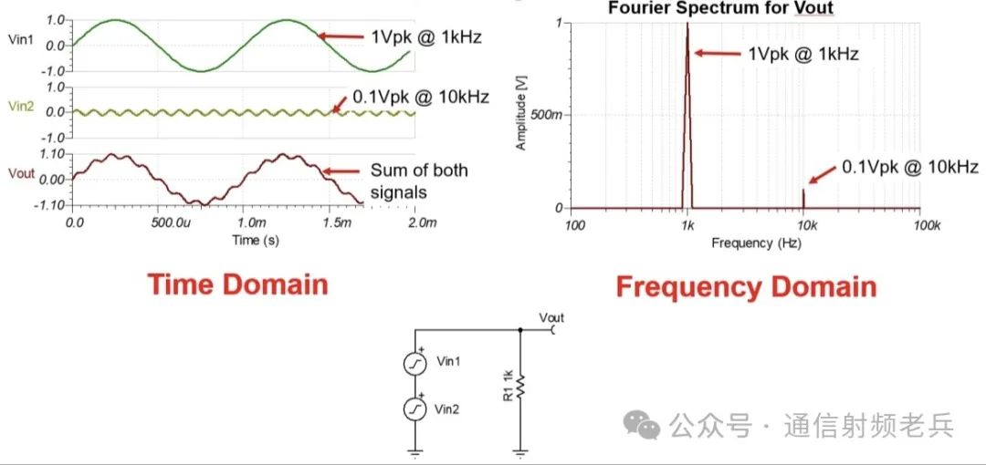
Here, we introduce the concepts of time domain and frequency domain. The time domain shows how the amplitude of a signal varies over time. In the time domain example, we create an unusual waveform by adding two sine waves. One is a sine wave with a peak voltage of 1V and a frequency of 1kHz, while the other is a waveform with a peak voltage of 0.1V and a frequency of 10kHz. We will observe this combined waveform in the frequency domain. In the frequency domain, the amplitude is on the vertical axis and the frequency is on the horizontal axis. The “Fourier spectrum” graph in the frequency domain always shows how the amplitude of the sine waveform varies with frequency. In this example, we are analyzing a signal Vout composed of two sine waveforms. Therefore, in the frequency domain, there are two components at 1kHz and 10kHz, with amplitudes of 1Vpk and 0.1Vpk, respectively. The key point here is that the frequency domain only displays the amplitude of the sine waveforms. So, how are non-sine waveforms displayed in the frequency domain?
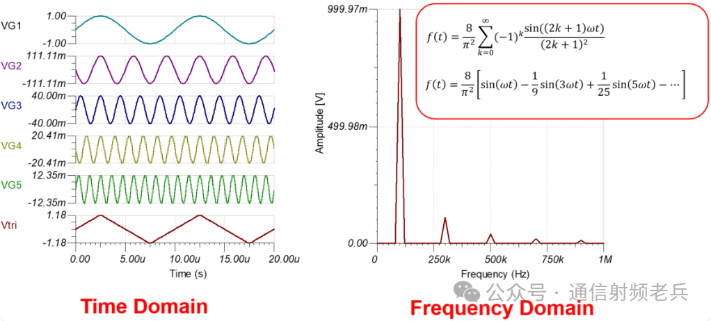
Any arbitrary waveform can be decomposed into an infinite series of sine waveforms. This infinite series is known as the Fourier series. Here is an example of the Fourier series of a triangular waveform. The mathematical function indicates that the series starts from sin(ωt), followed by 1/9sin(3ωt), 1/25sin(5ωt), and so on. The first and largest frequency component sin(ωt) is called the fundamental frequency. Subsequent sine components, such as sin(3ωt) and sin(5ωt), are called harmonics, and their amplitudes gradually decrease as the series continues. Theoretically, to perfectly represent a triangular waveform, an infinite number of sine waves are required. However, in practical operations, using the fundamental frequency and a few harmonics can represent the triangular waveform quite well. This example shows the fundamental frequency and four harmonics in both the time and frequency domains. Note the triangular waveform at the bottom of the time domain waveform; it is the direct sum of the above waveforms. The frequency domain of the triangular waveform is generated through a mathematical transformation called the Fourier transform. The Fourier transform is a general method for converting any time domain signal into its frequency domain equivalent.
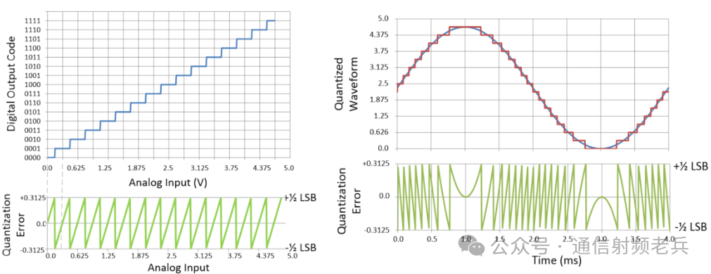
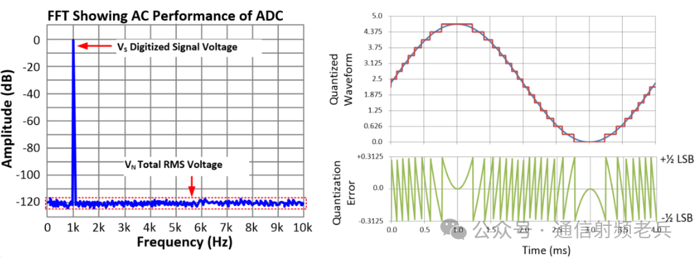
 The left side of the next figure shows an example of a four-bit transfer function. The horizontal axis represents the analog input signal, while the vertical axis represents the digital equivalent code. The digital output is a rounded version of the analog input. As the analog input voltage changes, it can be seen that each digital output code corresponds to a unique analog input value, at which point the error is zero. When the analog signal is above or below this value, the error increases or decreases, with the maximum error being half the least significant bit (LSB) width. This error caused by digital rounding is called quantization error. The right side shows a comparison between the digitized sine wave and the continuous analog input signal. The bottom of the page illustrates the quantization error of the sine wave. Quantization error can be viewed as a type of noise since it is superimposed on the digitized sine wave. The total root mean square (RMS) quantization noise can be determined by integrating the quantization error function. Next, let’s take a look at the frequency domain relationship of this waveform.
 On the left side of the next figure, you can see the frequency domain representation of the digitized sine wave. The applied digitized signal frequency is 1kHz, and the noise arises from the quantization noise caused by the “rounding” error on the waveform. Here, we consider an ideal data converter where all noise is derived from quantization noise. In practical situations, other noise sources also contribute to the noise floor. The total root mean square (RMS) quantization noise can be theoretically predicted by integrating the time domain quantization error waveform.
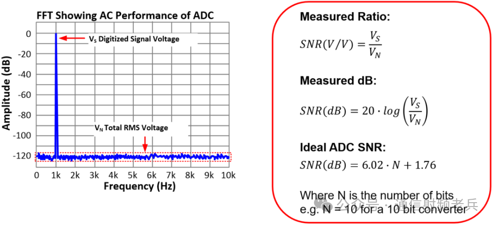
 The next figureshows the general formula for signal-to-noise ratio (SNR). Broadly speaking, the signal-to-noise ratio measures the purity of the signal or the noise level. A high SNR indicates that the signal is much larger than the noise, while a low SNR indicates that the noise is relatively high compared to the signal. In this ratio, both the signal and noise are measured in volts RMS. Taking the logarithm of this ratio and multiplying by 20 converts it to decibels (dB). The ideal signal-to-noise ratio (in decibels) can be calculated using the formula 6.02N+1.76, where N is the number of bits. For example, a 10-bit converter has an SNR of 60.2+1.76, which is 61.96dB. This relationship is derived by integrating quantization noise and applying the signal-to-noise ratio relationship. This is the signal-to-noise ratio relationship for an ideal converter (considering only quantization noise as a source of error). Due to the presence of other noise sources in practical converters, the SNR of any actual converter will never exceed the value given by this formula.
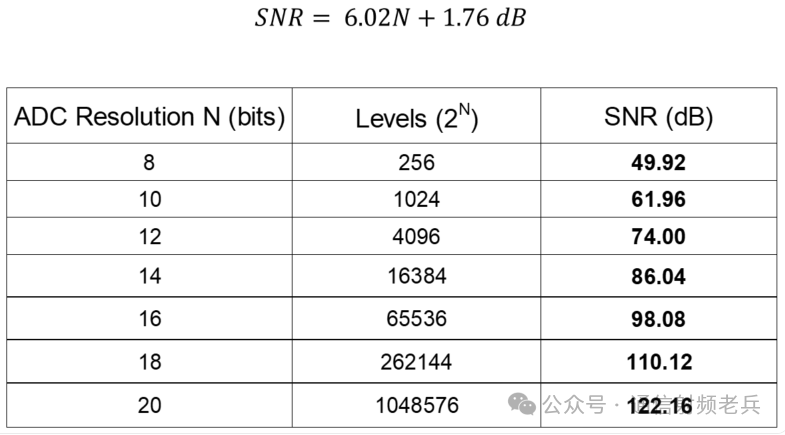
 This table lists the ideal signal-to-noise ratios (SNR) for various resolution analog-to-digital converters (ADC). The SNR values are calculated based on the formula SNR=6.02*N+1.76dB. For example, the ideal SNR for a 16-bit converter is 98.08dB. A practical 16-bit converter may approach an SNR of 98.08dB, but will never exceed this value. This formula and the associated table are a good way to understand how close a specific converter is to its ideal state.
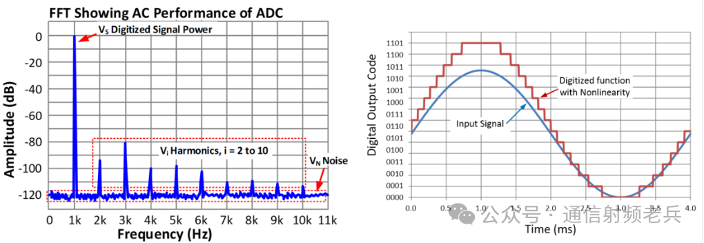
 In addition to the signal-to-noise ratio (SNR), total harmonic distortion (THD) is also a common metric in the AC specifications of data converters. To understand THD, it is crucial to comprehend nonlinearity. Nonlinearity is a measure of how much a transfer function deviates from its ideal linear form. The left side of the next figure shows a transfer function that includes both an ideal linear transfer function and a nonlinear transfer function. The ideal transfer function follows a straight line in the form of y=m*x+b, while the nonlinear transfer function includes higher-order terms, causing deviation from linearity. The shown nonlinearity example is exaggerated for easier observation of the nonlinearity. Note that the nonlinear function tracks well at low input levels but deviates as the input increases. In short, the gain for higher input signals exceeds the intended gain. This stretching of the upper half-cycle of the sine wave is called distortion and will produce harmonics in the frequency spectrum.
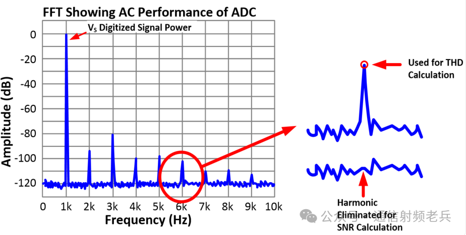
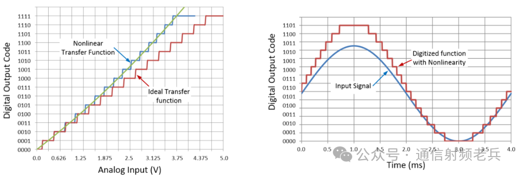 The next figure shows the frequency spectrum of the digitized sine wave on the right side. Harmonics are generated by the distortion of the upper half-cycle of the waveform. Harmonic distortion always occurs at integer multiples of the fundamental frequency. In this example, the fundamental frequency is 1kHz, and harmonics appear at 2kHz, 3kHz, 4kHz, etc. Sometimes it is useful to distinguish between even-order harmonics and odd-order harmonics because different circuit non-ideal factors may produce different types of harmonics. Even-order harmonics are multiples of the fundamental frequency, while odd-order harmonics are odd multiples of the fundamental frequency. In this example, 2kHz and 4kHz are even-order harmonics, while 3kHz and 5kHz are odd-order harmonics. If the digitized signal perfectly tracks the input signal, no harmonics would be produced.
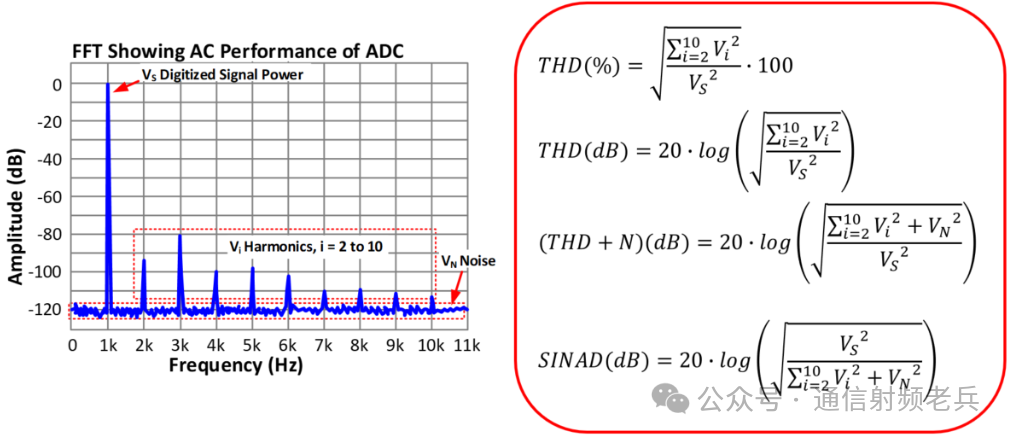
 The results of THD (Total Harmonic Distortion) are presented here in both percentage and decibel forms. The IEEE ADC testing standard specifies that THD should be calculated using harmonics from the second to the tenth. THD is the square root of the sum of the squares of the harmonic voltages divided by the square of the effective value of the signal voltage. This amount multiplied by 100 converts it to a percentage, or taking the logarithm and multiplying by 20 converts it to decibels. THD+N is similar to THD, except that it includes the total effective noise in its calculation. SINAD stands for Signal to Noise and Distortion Ratio. Mathematically, SINAD is the reciprocal of the THD+N calculation. In decibel units, taking the reciprocal only changes the sign of the value. Note that SINAD or THD+N is always worse than either THD or SNR alone, as SINAD is effectively a combination of both sources of error.
 It is important to note that when calculating SNR, the harmonic components included in the THD calculation are omitted. The harmonic components are replaced by the average noise at the frequencies where the harmonics occur. This is because distortion and noise are two different sources of error, and we do not want to include distortion in the noise calculation.