Where does the speed improvement of STM32 come from?
That’s right! The component that accelerates the image classification processing speed of STM32 is the Digital Signal Processor (DSP).
Currently, Arm‘s Cortex-M4, Cortex-M7, Cortex-M33, and Cortex-M35P microcontroller cores all come with DSP.
Compared to CPU (which excels at scheduling), DSP is very good at computations, handling complex operations in neural networks such as convolution and pooling, thus speeding up processing.
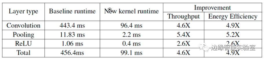
By adding DSP extensions to the Thumb instruction set and optional Floating Point Unit (FPU), the performance of numerical calculations has been improved. This not only allows for direct execution of signal processing operations on Cortex-M4, Cortex-M7, Cortex-M33, and Cortex-M35P processors but also maintains the ease of use of the Cortex-M programming model.
Looking at the arm_convolve_HWC_q7_RGB.c file in the project source code, you will find that STM32 uses __SIMD32 and __SXTB16 DSP instructions to improve computational speed.
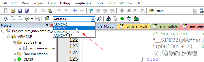
arm_status arm_convolve_HWC_q7_RGB(const q7_t * Im_in, const uint16_t dim_im_in, ... q7_t * Im_out, const uint16_t dim_im_out, q15_t * bufferA, q7_t * bufferB){ #if defined (ARM_MATH_DSP) /* Run the following code for Cortex-M4 and Cortex-M7 */ // Source code omitted... const q7_t *pPixel = Im_in + (i_ker_y * dim_im_in + i_ker_x) * 3; q31_t buf = *__SIMD32(pPixel); union arm_nnword top; union arm_nnword bottom; top.word = __SXTB16(buf); bottom.word = __SXTB16(__ROR(buf, 8)); // Source code omitted... #else /* Run the following code as reference implementation for Cortex-M0 and Cortex-M3 */ // Source code omitted... #endif /* ARM_MATH_DSP */ /* Return to application */ return (ARM_MATH_SUCCESS); }You can also experience the execution speed of the image classification application with and without DSP in the Keil simulator.
Memory Constraints
The memory of STM32 is very limited, for example, the STM32F427AG has only 256KB of memory. In the project source file arm_nnexamples_cifar10.cpp, two buffers col_buffer and scratch_buffer are created and reused between the layers of the neural network to reduce memory usage.
-
col_buffer stores the output of the convolution layer
-
scratch_buffer stores the output of intermediate layers
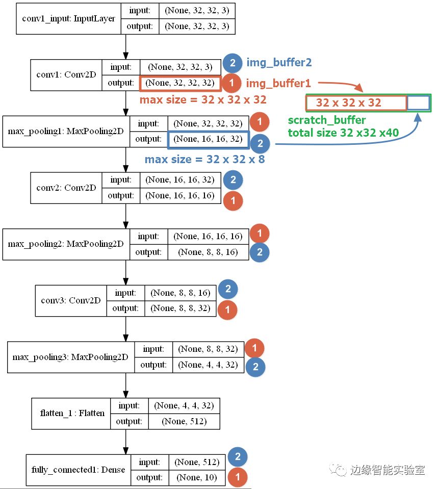
// typedef int8_t q7_t; // typedef int16_t q15_t; q7_t col_buffer[2 * 5 * 5 * 32 * 2]; q7_t scratch_buffer[32 * 32 * 10 * 4]; // Cut the scratch buffer to two buffers. q7_t *img_buffer1 = scratch_buffer; q7_t *img_buffer2 = img_buffer1 + 32 * 32 * 32; // conv2 img_buffer2 -> img_buffer1 arm_convolve_HWC_q7_fast(img_buffer2, CONV2_IM_DIM, CONV2_IM_CH, conv2_wt, CONV2_OUT_CH, CONV2_KER_DIM, CONV2_PADDING, CONV2_STRIDE, conv2_bias, CONV2_BIAS_LSHIFT, CONV2_OUT_RSHIFT, img_buffer1, CONV2_OUT_DIM, (q15_t *) col_buffer, NULL); arm_relu_q7(img_buffer1, CONV2_OUT_DIM * CONV2_OUT_DIM * CONV2_OUT_CH); // pool2 img_buffer1 -> img_buffer2 arm_maxpool_q7_HWC(img_buffer1, CONV2_OUT_DIM, CONV2_OUT_CH, POOL2_KER_DIM, POOL2_PADDING, POOL2_STRIDE, POOL2_OUT_DIM, col_buffer, img_buffer2);# 2*2*number of filters (convolution kernels)*kernel width*kernel height 2*2*(conv # of filters)*(kernel width)*(kernel height)These parameters can be found in the Caffe model, as shown in the figure below:

scratch_buffer is divided into two parts: img_buffer1 and img_buffer2. For a specific layer, one serves as input while the other serves as output. Its size can be determined by traversing the usage across layers.
max(img_buffer1)+max(img_buffer2) = 32*32*40Selecting the Right Convolution Layer Function
-
arm_convolve_HWC_q7_basic
-
arm_convolve_HWC_q7_fast
-
arm_convolve_HWC_q7_RGB
-
arm_convolve_HWC_q7_fast_nonsquare
Each of them is optimized for speed and size to varying degrees, but they also have different focuses.
arm_ve_HWC_q7_basic function is the most basic version, designed for any second-order tensor and weights of any dimension.
arm_ve_HWC_q7_fast function, as its name suggests, runs faster than the previous function, but requires the input tensor channels to be a multiple of 4 and the output tensor channels (number of filters) to be a multiple of 2.
arm_ve_HWC_q7_rgb is specifically built for convolution with an input tensor channel count of 3, typically applied to the first convolution layer with RGB image data as input.
arm_convolve_HWC_q7_fast_nonsquare is similar to arm_convolve_HWC_q7_fast, but can take non-square input tensors.
For fully connected layers, the two most distinct options are:
-
arm_fully_connected_q7
-
arm_fully_connected_q7_opt
The first uses a regular weight matrix, while the one with the suffix “_opt” is optimized for speed, but the layer’s weight matrix must be pre-sorted in an interleaved manner.
Conclusion
In this issue, we explained three key points of STM32 image classification applications: DSP acceleration, memory usage, and the selection of convolution layer functions. We hope this helps with your CMSIS-NN application development.

Embedded Machine Learning Series 00: STM32 Image Classification
Stop Searching! There’s No Clearer Explanation About Convolutional Neural Networks (CNN)!
Edge Intelligence Lab
Focusing on Edge Intelligence!
Long press to recognize the QR code to follow