 Paper Title
TGTM: TinyML-based Global Tone Mapping for HDR Sensors
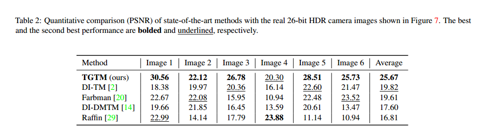
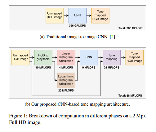
1 IntroductionAdvanced Driver Assistance Systems (ADAS) that rely on multiple cameras are becoming increasingly popular in vehicle technology.However, traditional imaging sensors struggle to capture clear images in conditions with strong lighting contrasts, such as at the exit of tunnels, due to their limited dynamic range.Introducing High Dynamic Range (HDR) sensors can address this issue.However, the process of tone mapping HDR content to a displayable range, when performed directly on pixel data, often results in inefficient computations.This paper focuses on HDR image tone mapping using a lightweight neural network applied to image histogram data.The proposed TinyML-based global tone mapping method, called TGTM, has a computational load of 9,000 FLOPS for RGB images of any resolution.Additionally, TGTM provides a universal approach that can be integrated into any classical tone mapping method.Experimental results show that TGTM outperforms state-of-the-art methods on real HDR camera images, achieving a PSNR improvement of up to 5.85 dB while reducing computational load by several orders of magnitude.This study demonstrates a computationally efficient tone mapping technique that uses CNNs to derive tone curve function parameters from image histograms.This type of research, particularly emphasizing the execution of machine learning (ML) models on embedded systems, is also known as TinyML.As shown in Figure 1, the method applies tone mapping to 26-bit HDR images and converts them to 12-bit LDR images.Given the use of supervised learning methods to train the machine learning model, a suitable data simulation method is also introduced to transition from a set of 8-bit sRGB images to unmapped linear HDR RGB images.Finally, the results of the simulated images are compared with available real data, and the results of real 26-bit images captured with HDR sensors are compared with manual tone mapping performed by our company’s image processing engineers.
2 Background
The dynamic range, defined as the ratio between the brightest and darkest perceivable light levels, is crucial for capturing accurate images.Image sensors commonly used in digital cameras, such as the one in the iPhone 15, have a dynamic range of about 70 dB.However, the intense glare from oncoming car headlights at night or the low sun on the horizon can blind such standard sensors.One method to extend dynamic range is to capture and fuse multiple exposures of different lengths into a single image.However, this can lead to ghosting artifacts with rapidly moving objects.As a result, HDR sensors with dynamic ranges of up to 140 dB have been developed to accurately address challenging environments in automotive applications.Cameras commonly used in automotive applications typically offer dynamic ranges between 70 and 140 dB.For example, the Sony IMX490 sensor specifically provides a dynamic range of 140 dB.
In a standard camera setup, a dedicated Image Signal Processor (ISP) is responsible for processing the captured sensor images to generate the final output image.Within the image processing pipeline, there are various steps, one of which is tone mapping.Tone mapping adjusts the intensity of input pixels to improve contrast and enhance the tones in the final image.Typically, the same tone mapping gain is applied to all three color channels (R, G, and B) of the image. Tone mapping can be achieved by either preserving the original dynamic range or exporting a low dynamic range (LDR) image from the HDR input image.This dynamic range compression is necessary to ensure compatibility with Standard Dynamic Range (SDR) displays.One of the focal areas of this paper is converting 26-bit HDR images to 12-bit LDR images.
There are two main approaches to applying tone mapping.The first is to create a single tone curve for the entire image, known as Global Tone Mapping (GTM).The second method estimates separate tone curves for different regions of the image, known as Local Tone Mapping (LTM).LTM is particularly effective in preserving local details.However, it can sometimes lead to halo artifacts and blocky areas, especially when there are significant differences in tone curves within the image.In contrast, GTM does not encounter these issues but lacks the ability to enhance local areas as effectively as LTM. Another approach to improve tone mapping is to use per-pixel enhancement techniques, typically implemented using Convolutional Neural Networks (CNNs).However, these methods often have high computational demands compared to those utilizing image statistics.
3 Proposed Solution
This work proposes a computationally efficient global tone mapping model designed to run on modern ISPs.Part of the project’s goal is to improve the automotive image processing pipeline IP (RPP) of Dream Chip using CNN algorithms while maintaining or minimally impacting processing latency.Additionally, it should demonstrate how to implement this ISP CNN method on the ZuSE-KI-Mobil SoC, regardless of whether modifications are made to the SoC design.Given the efficiency of the CNN method, requiring only 9k FLOPS, the algorithm can run on the application processing unit (APU) of the ZuSE-KI-Mobil SoC without the need for a dedicated CNN accelerator.
To avoid the burden of collecting and manually tone mapping training datasets, a data simulation method for supervised learning is introduced.This includes corresponding pairs of input images and ground truth tone curves.There are four key ideas in the proposed solution:
1. Data simulation using inverse tone mapping curves. Inverting the tone mapping curve and applying it to the image can automatically generate custom datasets.
2. Data compression using image histograms. Combining linear histograms and logarithmic histograms for data compression allows the method to handle information loss while maintaining resolution independence.
3. Curve parameter prediction. The method predicts not discrete tone curve values but rather curve parameters, which are passed to an analytical function to compute the curve. This ensures functional safety by utilizing known constraints and behaviors.
4. Curve integral loss. Introducing curve integral loss to mitigate bias in errors ensures higher accuracy.
3.1 Inference Process
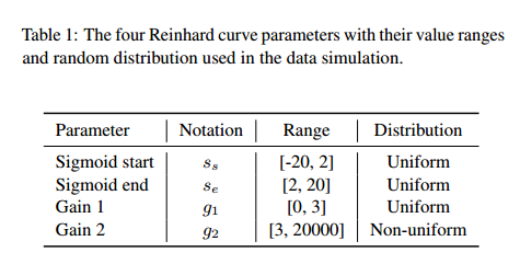
The complete process of tone mapping images is illustrated in Figure 2.The process takes an unmapped linear RGB HDR image as input, with a dynamic range of[0, 2 bits – 1].First, the image is converted to luminance space, and corresponding weights are assigned to the R, G, and B components [0.25, 0.50, 0.25]. Subsequently, a linear histogram is computed from this transformed image.In a parallel path, a logarithmic histogram is computed.Before performing logarithmic operations, the image needs to be converted to the same bit width used during training data simulation.This bit width conversion is crucial because logarithmic operations are nonlinear.However, in our case, this conversion is unnecessary as both processes use a 26-bit format.Then, both the linear and logarithmic histograms are input into the neural network, which predicts four parameters for creating the tone curve, as shown in Table 1.
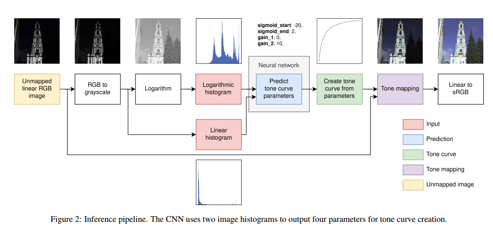
The tone curve is created using an improved Reinhard formula.

Wherex is the input value between0 andm is the maximum value used for the curve, for example,2 bits – 1 andg is the gain. The equation is an extension of Reinhard’s, adding a scaling factor to keep white as white.Similarly, 0 ensures0 ≤ci ≤m.The final tone curve is created by mixing two such curvesc1 andc2 to enhance tone mapping in images with bright and dark parts.The mixing is completed using the weights of the sigmoid curves(ss, se) wheress is the starting value of the sigmoid,se is the ending value of the sigmoid.The tone curve is shown below

Wheres is the sigmoid value at pointx andc1 andc2 are the gain curves evaluated at pointx with gainsg1 andg2.If the mixing produces a negative slope, it is replaced with a horizontal line starting from the top point and ending at a point above the horizontal line.This fixes unnatural results that may occur due to the inversion of the tone range.Finally, tone mapping (including the conversion from 26 bits to 12 bits) is applied to the unmapped image, which is then converted to the sRGB domain.
3.2 Data Simulation
A robust tone mapping dataset should avoid relying on individual preferences for tone mapping.Moreover, the accuracy of tone mapping should not be limited by the use of existing tone mapping algorithms to generate ground truth data.Two public datasets were evaluated: the HDR+ dataset and MIT-Adobe FiveK.The HDR+ dataset provides metadata for each image, including the tone mapping curves used to process the raw images.However, this is not sufficient, as we do not want to limit our capabilities and ideally reach the level of existing tone mapping algorithms.On the other hand, MIT-Adobe FiveK employed five photography students from an art school to adjust the tones of the photos.While this method provides human input, it is not ideal as it involves local adjustments to the images, making it challenging to accurately estimate a single tone curve between two images.Therefore, it is recommended to simulate a dataset without relying on existing algorithms and without requiring human input during the adjustment process.
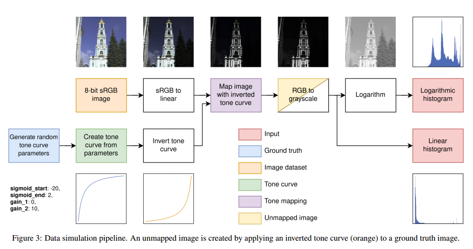
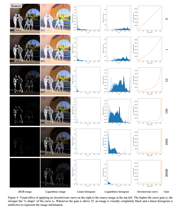
In image enhancement projects, a typical data simulation method is to create input images by adding degradations to high-quality real images.In Figure 3, an 8-bit sRGB image selected from the MIT-Adobe FiveK dataset is converted to a 26-bit format to reduce quantization errors in subsequent processing steps and an inverse gamma curve is applied to obtain linear RGB data.Simultaneously, in another branch, a random tone curve is generated using Equation 2.The four parameters used in the curve creation are randomly selected, except for the gain2 parameter, which follows a uniform distribution within a defined range.These parameters are shown in Table 1.Due to the nonlinear relationship between the gain2 parameter and the shape of the curve, it exhibits non-uniform randomness.Using uniform randomness would lead to an average gain value of about 10k, primarily composed of images from extremely dark scenes.Therefore, to ensure equal representation of bright and dark scenes, randomness is applied in the logarithmic domain.The effect of gain is illustrated in Figure 4.
The tone curve is created according to Equation 2 and then inverted.Subsequently, the image is tone mapped using the inverted tone curve and then converted to luminance space.Finally, two histograms are computed from the luminance image.
Given the wide dynamic range involved, most pixel values fall within the visually dark areas.To demonstrate the effect of the tone curve gain, see Figure 4.It illustrates the complete dynamic range used during data simulation.Additionally, it emphasizes the necessity of using logarithmic histograms to avoid information loss in linear histograms.
3.3 Neural Network Structure
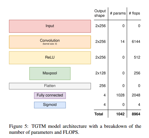
The neural network architecture is shown in Figure 5.The input is a stacked tensor of 2×256-bin histograms.This arrangement ensures that the histogram aligns with the corresponding elements during the convolution process.The histogram is normalized to ensure consistent performance regardless of image resolution.
Calculating the Mean Absolute Error (MAE) from the four parameters in Table 1 is effective, but relying solely on it introduces bias in the loss.Given the strong nonlinear relationship between the value of the parameterg2 and the shape of the corresponding gain curvec2, it is recommended to also compute the loss fromc2 using Equation 1 to mitigate bias.To improve efficiency, it is suggested to compute the curve loss between the predicted and true values ofc2 gain curves, referred to as Curve Integral Loss (CIL).Thus, during training, the cost function includes a combination of MAE and CIL.
The predicted output includes four values used in Equation 2 to create the tone curve.This method performs better than estimating discrete curve values.Additionally, by predicting curve parameters, it ensures consistency of all possible curve shapes, smooth transitions across frames, and the ability to generate curves with any number of steps, even if the steps are not equal.The curve is always generated within a fixed range from 0 tom or generating curves from the minimum to maximum capture values of the image may yield better single-image tone mapping.However, it alters the range of image values, making the algorithm more susceptible to temporal inconsistencies, such as flickering lights.For video capture use cases, it is recommended to generate curves for the entire value range to achieve better temporal stability.
3.4 Computational Complexity
The proposed network structure is compact, containing only 1,042 parameters and requiring 8,964 floating-point operations. The CNN requires only 0.3% of the model parameters used in DI-TM (340,227 parameters and 366 GFLOPS).However, when comparing floating-point operations, the entire process of TGTM must be considered. Given the demand for efficient memory and computation when applying tone mapping, creating tone curves for the entire value range of [0, 2^26 – 1] (including 67 million values) is impractical.Therefore, it is chosen to create a non-equidistant piecewise linear tone curve with 49 sampling points and interpolate the remaining values during tone mapping.
Evaluating the total cost of calculating 49 tone curve sampling points using Equation 2 takes less than 3,000 FLOPS.Since this computation is performed only once per image and runs in parallel with the CNN, its impact is negligible compared to the FLOPS applied to pixel data, effectively approximating to 0 FLOPS per pixel.As a reference, the runtime of the exported CNN model and tone curve creation C code on a Raspberry Pi 1 is 994 μs, while on a Raspberry Pi 4 it is 53 μs.However, for the proposed tone mapping, the cost of applying the tone curve to pixels is 12 FLOPS. Additionally, as shown in Figure 1, converting RGB images to grayscale and computing linear and logarithmic histograms costs 5, 2, and 10 FLOPS per pixel, respectively.While DI-TM requires 176,614 FLOPS per pixel, our overall cost is much lower, totaling 29 FLOPS per pixel.Ultimately, compared to the portion of processing pixel data, the thousands of FLOPS in our CNN and tone curve creation can be considered negligible, making the proposed CNN method computationally feasible for any ISP.
3.5 Training Details
The training dataset is MIT-Adobe FiveK.It contains 5,000 images with varying resolutions, orientations, and image content.The training data is simulated by applying six random inverse tone curves to each image, resulting in 30,000 training samples.The validation data is simulated by applying a single random inverse tone curve to 2,000 images.In the simulation, following the process in Figure 3, the 2×256 input histogram and four ground truth parameters are saved in a text file.It completes in 15 minutes on a single thread of an AMD Ryzen Threadripper PRO 3975WX CPU.
The batch size used is 16, resulting in 1,875 iterations per epoch.The optimizer is Adam, with a learning rate of 1e-4.The scheduler used, ReduceLROnPlateau, is set to reduce the learning rate based on validation set loss stagnation, with a reduction factor of 0.3 until a minimum of 1e-8, with a patience value of 6 epochs.The final model was achieved after 97 epochs (181,875 iterations).Development was completed using the Pytorch framework, with a total training time of 7 minutes on a single Nvidia A6000 GPU.
3.6 Solution Constraints
The proposed solution has some limitations that affect its performance.First, compared to LTM methods, GTM performs poorly on high-contrast images.Second, consistency in bit width between data simulation and inference is necessary; if different bit widths are used, conversion or retraining is required.Third, a dedicated image histogram computation module is required in the ISP.
4 Experiments
1) Visual comparison of state-of-the-art methods using real-world 26-bit unmapped images
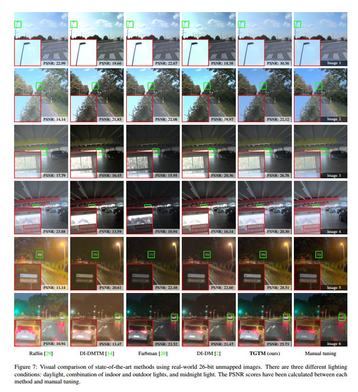
2) Figure 7 shows a quantitative comparison of the latest methods with real 26-bit HDR camera images (PSNR).