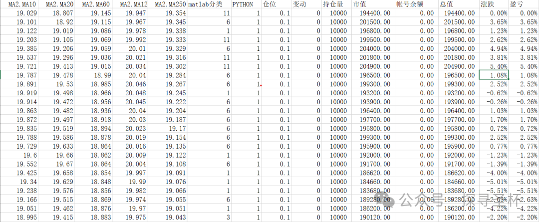
A clustering analysis is performed on a vector composed of the closing prices of stocks and several important moving average prices, attempting to identify trend characteristic classifications, which can serve as a basis for position management. The following code has been debugged using Spyder, but the classification results are not ideal, and different parameters need to be tried. For practice, here is the record:
# -*- coding: utf-8 -*-
“””
Spyder Editor
This is a temporary script file.
“””
from minisom import MiniSom
import numpy as np
import pandas as pd
data = np.loadtxt(‘D:\Programming Practice\gpfx.csv’, delimiter=’,’, skiprows=1, usecols=(1,2,3,4,5,6,7), unpack=False)
# data normalization
data = (data – np.mean(data, axis=0)) / np.std(data, axis=0)
# Initialization and training
som_shape = (3, 4)
som = MiniSom(som_shape[0], som_shape[1], data.shape[1], sigma=0.6, learning_rate=.5,
neighborhood_function=’gaussian’, random_seed=10)
som.train_batch(data, 2000, verbose=True)
# each neuron represents a cluster
winner_coordinates = np.array([som.winner(x) for x in data]).T
# with np.ravel_multi_index we convert the bidimensional
# coordinates to a monodimensional index
cluster_index = np.ravel_multi_index(winner_coordinates, som_shape)
import matplotlib.pyplot as plt
# plotting the clusters using the first 2 dimensions of the data
for c in np.unique(cluster_index):
plt.scatter(data[cluster_index == c, 0],
data[cluster_index == c, 1], label=’cluster=’+str(c), alpha=.7)
# plotting centroids
for centroid in som.get_weights():
plt.scatter(centroid[:, 0], centroid[:, 1], marker=’x’,
s=80, linewidths=35, color=’k’, label=’centroid’)
plt.legend();