Breaking down auditory perception into data, and letting the ESP32 recognize the sound world! This project fully builds an environmental sound classification system using the ESP32-S2-Mini-1: from microphone audio capture, to window function + RFFT for frequency spectrum transformation, followed by Mel feature extraction and lightweight CNN inference, ultimately displaying scene categories such as “rain sound” and “dog barking” on the onboard OLED. Embedded “auditory intelligence” is at your fingertips, starting with AI from sound.
1
Introduction

1.1 Module/Chip Introduction
This project uses the ESP32-S2-Mini-1 module from Espressif Systems. The ESP32-S2-MINI-1 is a versatile Wi-Fi MCU module with powerful features and rich peripheral interfaces, suitable for applications in wearable electronics, smart homes, and more. The main specifications are as follows:
-
Core: Xtensa® single-core 32-bit LX7 CPU, frequency up to 240MHz
-
Memories:
-
128 KB of ROM
-
320 KB of SRAM
-
16 KB of RTCSRAM
-
4 MB of Flash memory
For more information, please refer to:
https://www.eetree.cn/doc/detail/2298
1.2 Development Board Introduction
This project uses an audio development board designed with the above module provided by Hehe Academy, integrating the following peripheral circuits and functions:
-
Based on the ESP32-S2 WiFi core module
-
128*64 OLED display, SPI interface, for displaying information, parameters, and waveforms
-
4 buttons for parameter control and menu selection
-
1 Mic audio input – analog circuit, with a potentiometer to adjust gain from 0-40dB, and a bandpass filter
-
1 headphone jack audio input – analog circuit, with a potentiometer to adjust gain from 0-40dB, and a bandpass filter
-
2 audio outputs with power amplification, capable of driving speakers and headphone jacks
-
An FM receiver module, with parameters set via I2C interface by the ESP32, to adjust FM stations and volume
-
A switch to toggle between audio generated by the ESP32 and FM output, with the module’s output sent to the speaker or headphone output
For more information, please refer to:
https://www.eetree.cn/project/detail/419
1.3 Task Introduction
Audio Scene Classification (ASC) is a fundamental task in the field of computer acoustics. Its goal is to correctly classify a segment of captured audio into corresponding environmental labels, such as dog barking or rain. This project implements embedded deployment of ASC on the ESP32 platform, allowing it to operate with low power in our daily lives. This project will introduce the various processes involved in implementing audio scene classification using the ESP32, including data collection, feature extraction, neural networks, and implementation methods.
2
Data Collection

Observing the schematic, we can see that the signal received by the Mic is amplified by the operational amplifier U9, and the gain can be adjusted via RV1, ultimately connecting to the ESP32 ADC input. Therefore, the collection part uses DIG ADC1 at a sampling rate of 20kHz to measure the voltage at the pin, and directly copies it to memory via DMA (Direct Memory Access) without CPU processing. The driver for this part directly uses the project-developed code, but due to API updates, I forcibly used deprecated library functions, resulting in warnings during compilation. This part of the driver can be upgraded in the future.
https://www.eetree.cn/project/detail/537
3
Feature Extraction

Feature extraction is the most crucial step for audio perception. The ultimate goal of this part is to convert a segment of audio close to one second into a 30×30 spectrogram. Next, I will explain how to generate a column of data in this spectrogram:
3.1 Window Function
First, we extract 1024 consecutive points from the sampled audio data. These points will subsequently undergo Fourier transformation. Before that, to reduce spectral leakage, we multiply this segment of data by a function that is large in the middle, maximum at 1, and gradually approaches 0 at both ends, known as a “window function.” I used the commonly used Hanning window, which can be referenced here:
https://numpy.org/doc/stable/reference/generated/numpy.hanning.html
3.2 Fast Fourier Transform
Next, we perform a Fast Fourier Transform on these 1024 points. This means that the original signal’s horizontal axis is time, reflecting the signal’s intensity at different times. After transformation, we obtain the distribution of energy of the audio over various frequencies during that time period. As shown in Figure 3.1(a), the left red signal is the time-domain signal before transformation, while the right shows the energy distribution in the frequency domain after transformation. If you are unfamiliar with Fourier transformation, I highly recommend this popular science video:
https://www.bilibili.com/video/av19141078
For the implementation part, I referred to the open-source code for Real FFT (RFFT):https://github.com/willhope/Noise-reduction/blob/master/rfft.c
3.3 Mel Spectrum
Research shows that human perception of frequency is not linear, and we are more sensitive to low-frequency signals than to high-frequency signals. For example, people can easily distinguish between 500 and 1000Hz, but it is quite difficult to notice the difference between 7500 and 8000Hz. However, the horizontal axis of the spectrum after Fourier transformation is linear. At this point, the Mel scale is proposed, which is a nonlinear transformation of Hz. For signals measured in Mel scale, it allows for nearly equal perception of frequency differences. The right side of Figure 1 shows the relationship between human perception of pitch and their actual frequencies. For more information, please refer to:
https://zhuanlan.zhihu.com/p/351956040
In this project, I used 30 sets of filters, so the original array length of 1024 becomes 30 after transformation. During implementation, I referred to and ported the official STM32 audio processing library, which includes common functions for feature extraction, such as Fourier transformation and Mel spectrum. Since ST uses ARM’s DSP to accelerate floating-point operations, when porting to ESP32, I had to replace all with standard mathematical functions, manually adding implementations for missing functions, and finally resolving various compilation issues, which took considerable effort. The address for ST’s audio processing library is:
https://www.st.com/zh/embedded-software/fp-ai-sensing1.html
It is worth mentioning that ESP also has a DSP library, but due to time constraints, I couldn’t study it in detail.
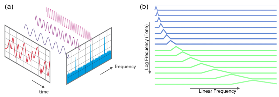
Figure 1 Fourier Transformation and Mel Spectrum
3.4 Program Flow
As shown in Figure 2, to enable the program to implement the above process, I first created 6 DMA receive buffers of length 256 uint16. When an interrupt occurs, the data of the previous 1024 points is extracted and normalized to floating-point numbers, performing a Fast Fourier Transform to obtain the Fourier spectrum. Then, a length of 30 array is calculated as a column of the Mel spectrum. Every 512 sampling points, a column of the Mel spectrum is calculated from the 1024 points. Once 40 columns of results are calculated, this data can be used for subsequent classification.
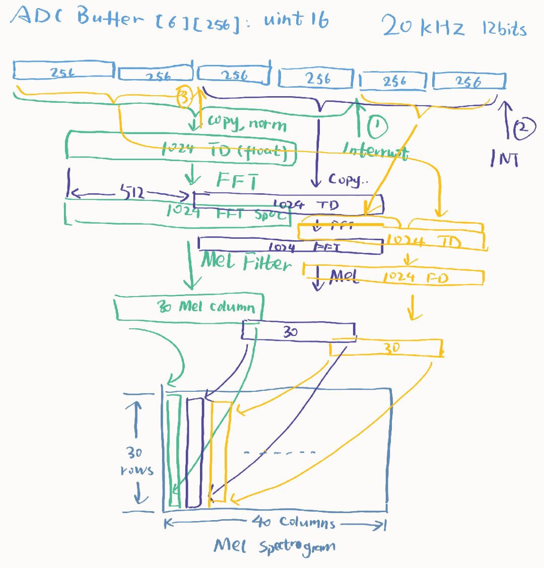
Figure 2 ESP32 Signal Processing Flowchart
4
Model Training

Model training is completed on a personal computer using Python scripts and the Pytorch deep learning framework.
4.1 Dataset
We used the ESC-10 dataset as training data. ESC stands for Environmental Sound Classification, and ESC10 contains 10 audio categories, each with 40 audio segments. The dataset download link is:
https://dataverse.harvard.edu/dataset.xhtml?persistentId=doi:10.7910/DVN/YDEPUT
Additionally, commonly used datasets include UrbanSound8k, etc. After downloading, we use the aforementioned feature extraction process to obtain the spectrogram for each audio segment. However, in the Python environment, using the librosa library, only two lines of code are needed to perform Fourier transformation and Mel spectrum operations.
4.2 Model Structure
After feature extraction, the audio classification problem is transformed into an image classification problem. We use a relatively simple CNN convolutional neural network for classification. Due to the limited memory on the ESP32 platform and the fact that Hehe uses a chip model without 2M PSRAM, which only has 320k of built-in SRAM, the network size cannot be too large. Generally, in embedded platforms, memory size limits the network scale, while CPU performance determines how fast the network can run. For visualizing the CNN model structure, I recommend referring to the following website:
https://poloclub.github.io/cnn-explainer/
5
Model Deployment

After training the model, the same CNN model structure can be implemented in ESP32 using C language. Then, parameters from the trained Pytorch model can be exported and compiled into the program as arrays, achieving model deployment. The ESP official also launched a more advanced deep learning library that can directly convert and deploy trained models, providing a series of tools. However, due to personal time constraints, I still wrote my own model inference code.
6
Program Flowchart

The program retains functions such as DAC signal generator, as it uses the previous author’s code as a framework. The specific operations are as follows:
Button 1: DAC switch (valid when ADC is off); ADC digital filter parameter settings (valid when ADC is on)Button 2: ADC switch (valid when DAC is off)Button 3: When ADC is on: ADC mode adjustment (detailed in the following text); when DAC is on: DAC volume adjustmentButton 4: DAC frequency switch
Figure 3 focuses on the program logic during ADC mode. When ADC is turned on, the ADC_Task task will start executing and continuously respond to ADC DMA interrupts. Then, it executes the corresponding code based on one of the four modes selected by the ADC button.
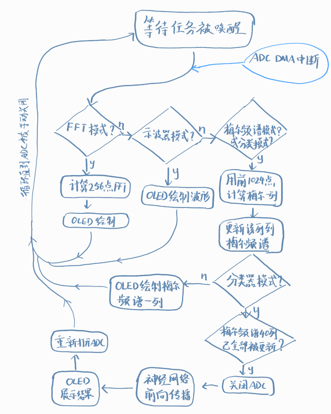
Figure 3 Program Execution Flowchart in ADC Mode
7
Key Code

The code for the neural network inference process is as follows, reflecting the structure of the neural network. The functions called in the code are self-implemented C language functions for convolution, pooling, etc.
xSemaphoreTake( xMutexSpec, portMAX_DELAY );conv2d_relu(&spec, 1, 30, 40, feature1, 10, conv1_1_w, conv1_1_b);xSemaphoreGive( xMutexSpec );conv2d_relu(feature1, 10, 28, 38, feature2, 10, conv1_2_w, conv1_2_b);swap_feature(feature1, feature2);max_pool2d(feature1, 10, 26, 36, feature2);swap_feature(feature1, feature2);conv2d_relu(feature1, 10, 13, 18, feature2, 10, conv2_1_w, conv2_1_b);swap_feature(feature1, feature2);conv2d_relu(feature1, 10, 11, 16, feature2, 10, conv2_2_w, conv2_2_b);swap_feature(feature1, feature2);max_pool2d(feature1, 10, 9, 14, feature2);swap_feature(feature1, feature2);flatten_fc(feature1, 10, 4, 7, out_neurons, 10, fc_w, fc_b);The neural network inference code trains for 10 epochs, with about 2000 one-second sound segments per epoch, and a batch_size of 10.
for epoch in range(num_epochs): # loop over the dataset multiple times running_loss = 0.0 correct = 0 for i, data in enumerate(asc_dataloader, 0): # get the inputs; data is a list of [inputs, labels] inputs, labels = data labels = torch.tensor(labels, dtype=torch.long) # zero the parameter gradients optimizer.zero_grad() # forward + backward + optimize outputs = model(inputs) loss = criterion(outputs, labels) loss.backward() optimizer.step() _, preds = torch.max(outputs, 1) # show_images(inputs[:6], labels[:6], preds[:6]) correct += (preds == labels).sum() # print statistics running_loss += loss.item() if i % 1 == 0: # print every 2000 mini-batches print('Epoch [{}/{}], Step [{}/{}], Loss(Avg): {:.3f}' .format(epoch + 1, num_epochs, i + 1, len(asc_dataloader), running_loss / 1)) running_loss = 0.0 print("Epoch {}, Acc: {}/{}".format(epoch + 1, correct, asc_dataset.__len__())) correct = 08
Results

The final experimental phenomenon is that after powering on the board, it continuously collects audio data, and then displays the classification results and probabilities on the OLED screen, as shown in Figure 4.
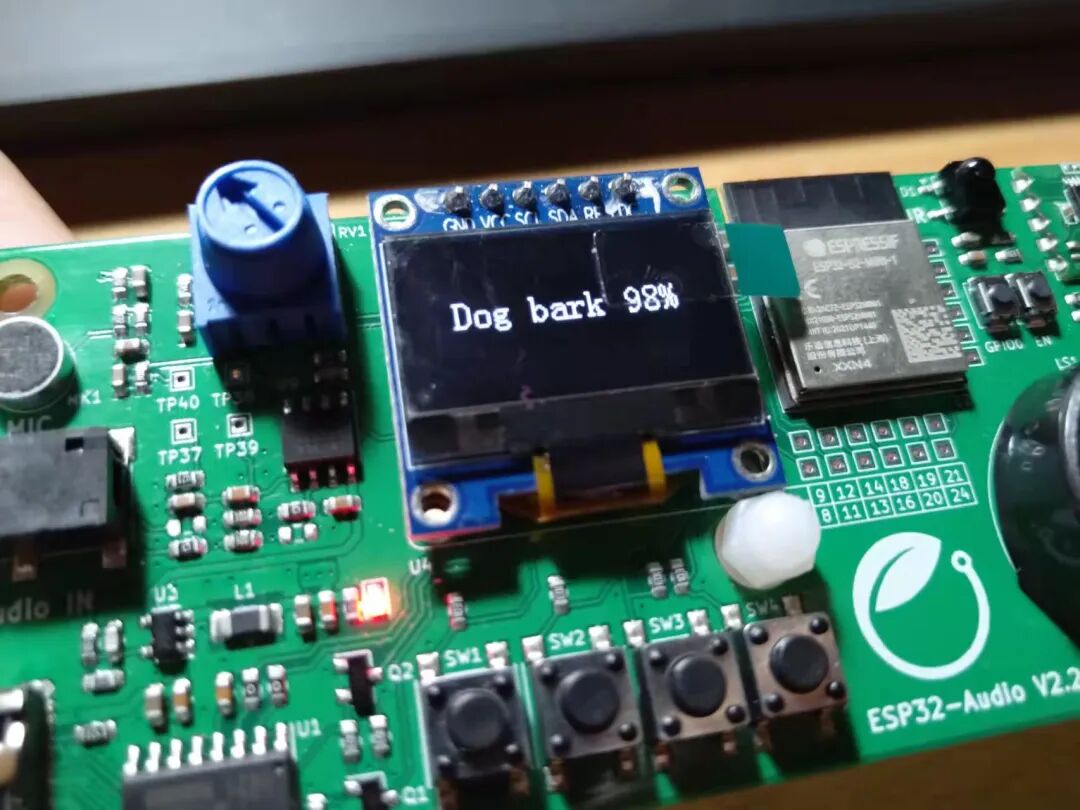
Figure 4 Physical Result DisplayThis audio classification case is entirely based on the ESP32-S2-Mini-1 implementation. If you want to explore embedded AI at home, you might as well start with this small board. It is already available in the Little Footstep Enterprise Store, interested students can directly purchase it and learn while practicing.

Click “Read the original text” to view the project