Click the blue text above to follow us

0
Gift to readers
👨💻 Engaging in scientific research involves a deep-seated system of thought, requiring researchers to be logical, meticulous, and earnest. However, it’s not just about hard work; many times leveraging resources is more important than effort. Additionally, having innovative insights and inspirations is crucial. Readers are advised to browse in order to avoid suddenly falling into a dark maze without finding their way back. This article may not reveal all the answers but can help clarify some doubts that arise in your mind, potentially creating a vibrant sunset of understanding. If it brings you a storm in your spiritual world, take the opportunity to brush off the dust that has been lying on your ‘lying flat’ mindset.
Perhaps, after the rain, the world will be clearer…🔎🔎🔎

01
Overview
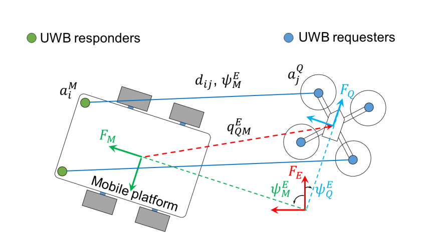
Abstract — This paper proposes a method for achieving relative positioning and tracking of quadrotors using ultra-wideband (UWB) ranging sensors, which are strategically installed to assist in retrieving the relative position and bearing between the quadrotor and the target. To achieve robust autonomous flight localization even in the presence of uncertainties, there are two main features. First, an estimator based on the Extended Kalman Filter (EKF) is developed to fuse UWB ranging measurements with onboard data from sensors, including Inertial Measurement Units (IMU), barometers, and optical flow. Second, to properly handle the target’s orientation and distance measurements, the communication capability of UWB is utilized to transmit the direction of the target quadrotor. Experimental results demonstrate the quadrotor’s ability to control its position relative to the following objects when the target is stationary, in both autonomous and mobile scenarios. UWB robust relative positioning and ranging.
In multi-robot systems, it is typically expected that each robot can determine its relative position to other robots to perform tasks such as UGV-MAV (Unmanned Ground Vehicle-Micro Air Vehicle) collaboration or formation movement. In such scenarios, a common approach is to assume that each robot can determine its position within a globally shared framework and transmit this information to its neighbors. However, satellite-based systems, such as GPS (Global Positioning System), are limited to open and tidy outdoor environments. Alternative methods, such as motion-tracking camera systems or radio-based positioning systems, rely on careful setup in the operational area. Examples of the latter include our previous work based on UWB positioning [1],[2],[3] and similar works in other literature [4],[5]. Alternatively, some works assume a certain proximity sensing capability. One method is to use distance sensing techniques, such as infrared distance sensors [6] or laser scanners [7]. However, this approach cannot provide identification of neighbors over relatively short ranges. Another promising approach has been the use of computer vision systems, which provide a favorable alternative for the proposed system, though it is not without limitations. See [8],[9], etc., [10]. In summary, its limitations include a limited field of view, short range, and potentially high computational requirements that lightweight aerial robots may not meet. In this paper, we propose a single-target relative positioning system for a single mobile robot. Here, we utilize UWB-based TWTOF (Two-Way Time of Flight) asynchronous ranging measurements for the target mobile robot to determine relative position without additional external devices. The position estimation method is similar to our previous work in the literature [11] and [2]. Instead of placing multiple anchor points in the operational area, both robots carry multiple UWB antennas placed in an appropriate configuration. Additionally, we developed the system for MAV-UGV cooperative scenarios (Figure 1) and integrated IMU, barometric, and optical flow data into the Extended Kalman Filter to provide sufficiently accurate and stable relative position data for feedback control of flight. This ranging-based method is omnidirectional and allows other sensors (such as cameras) to be used for other tasks rather than being trained for the target [12]. Using this system, the MAV will be able to accurately locate itself around the unmanned ground vehicle, perform tasks, and dock precisely. For such applications, UGVs can be assumed to remain fixed; however, in this work, we focus on testing the system’s robustness when the target is moving and the MAV is unaware of its speed. Detailed articles can be found in Section 4.

02
Operating Results
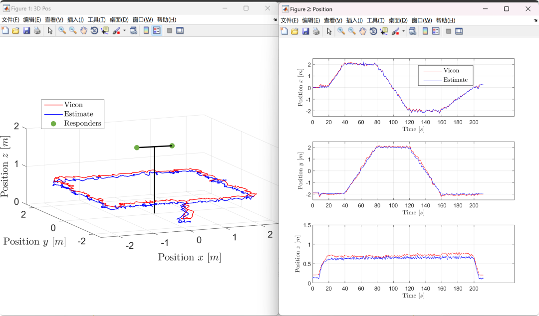
Visualization part of the code:
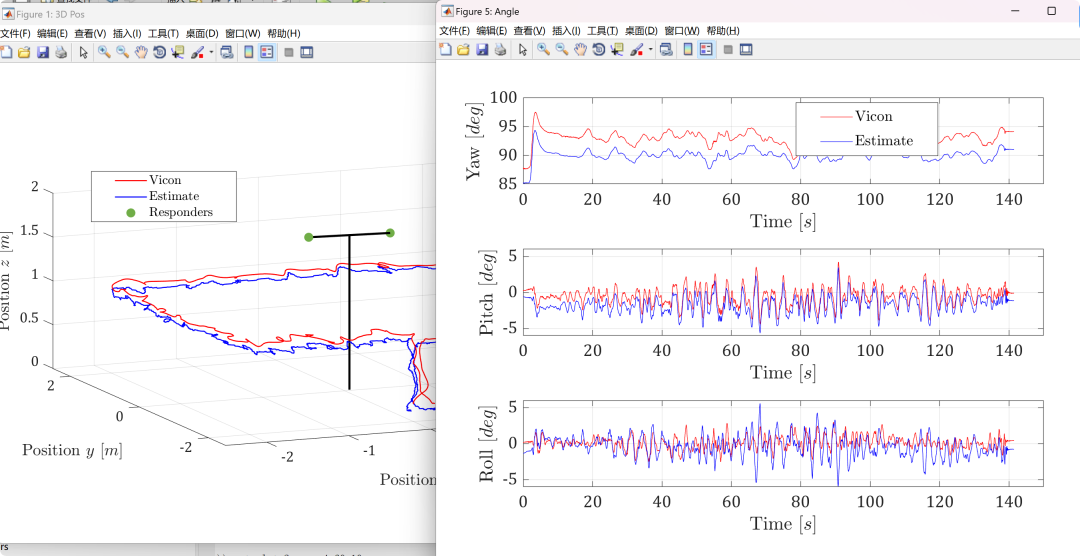
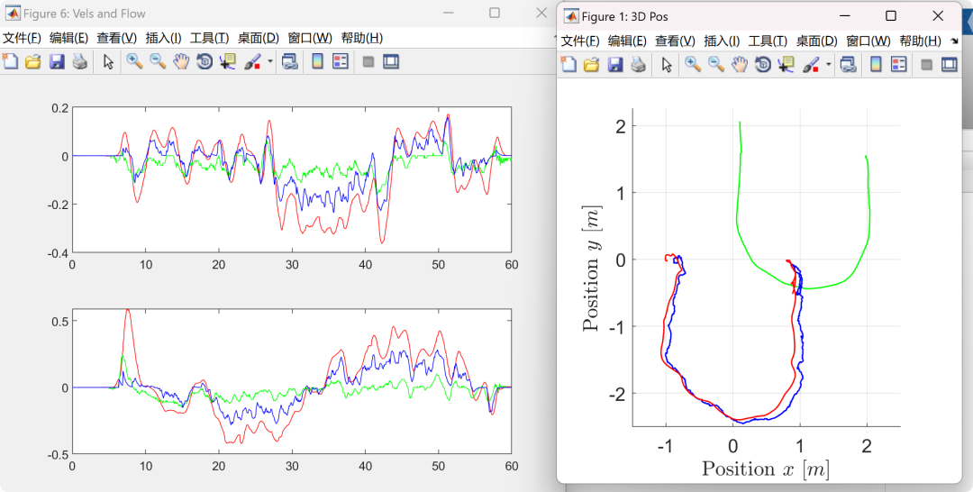
figure('name', '3D Pos', 'position', [865 200 400 400], 'color', [1 1 1]);
hold on;
vctarhd = plot3(vcTarP(1, :), vcTarP(2, :), vcTarP(3, :), 'g', 'linewidth', 1);
vcquadhd = plot3(vcP(1, :), vcP(2, :), vcP(3, :), 'r', 'linewidth', 1);
px4quadhd = plot3(px4P(1, :), px4P(2, :), px4P(3, :), 'b', 'linewidth', 1);
set(gca, 'DataAspectRatio', [1 1 1], 'fontsize', 14);
xlim([-1.5, 2.5]);
ylim([-2.5, 2.25]);
ylb = ylabel('$\mathrm{Position}\ y\ [m]$', 'interpreter', 'latex');%, 'position', [-9.2995 -14.2466 2.6102]);
xlabel('$\mathrm{Position}\ x\ [m]$', 'interpreter', 'latex');
zlabel('$\mathrm{Position}\ z\ [m]$', 'interpreter', 'latex');
grid on;
figure('name', 'Position','position', [1278 100 840 630], 'color', [1 1 1]);
subplot(3, 1, 1);
plot(t, vcP(1, :), 'r', t, px4P(1, :), 'b');
grid on;
set(gca, 'XTick',t(1):20:t(end));
xlabel('$\mathrm{Time}\ [s]$', 'interpreter', 'latex', 'fontsize', 14);
ylabel('$\mathrm{Position}\ x\ [m]$', 'interpreter', 'latex', 'fontsize', 14);
lghd = legend('$\mathrm{Vicon}$', '$\mathrm{Estimate}$');
set(lghd, 'interpreter', 'latex', 'fontsize', 14, 'position', [0.5360 0.8102 0.2117 0.1057]);
set(gca, 'fontsize', 16);
grid on;
subplot(3, 1, 2);
plot(t, vcP(2, :), 'r', t, px4P(2, :), 'b');
grid on;
set(gca, 'XTick',t(1):20:t(end));
xlabel('$\mathrm{Time}\ [s]$', 'interpreter', 'latex', 'fontsize', 14);
ylabel('$\mathrm{Position}\ y\ [m]$', 'interpreter', 'latex', 'fontsize', 14);
set(gca, 'fontsize', 16);
subplot(3, 1, 3);
plot(t, vcP(3, :), 'r', t, px4P(3, :), 'b');
grid on;
set(gca, 'XTick',t(1):20:t(end));
xlabel('$\mathrm{Time}\ [s]$', 'interpreter', 'latex', 'fontsize', 14);
ylabel('$\mathrm{Position}\ z\ [m]$', 'interpreter', 'latex', 'fontsize', 14);
set(gca, 'fontsize', 16);
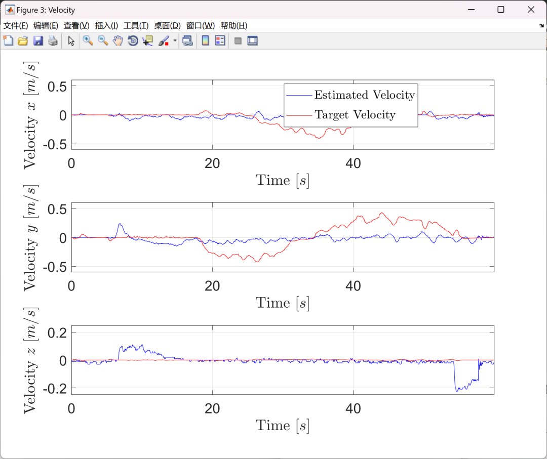
figure('name', 'Velocity','position', [1278 100 840 630], 'color', [1 1 1]);
subplot(3, 1, 1);
plot(t, px4V(1, :), 'b', t, vcTarV(1, :), 'r');
grid on;
ylim([-0.6, 0.6]);
set(gca, 'XTick',t(1):20:t(end));
xlabel('$\mathrm{Time}\ [s]$', 'interpreter', 'latex', 'fontsize', 14);
ylabel('$\mathrm{Velocity}\ x\ [m/s]$', 'interpreter', 'latex', 'fontsize', 14);
lghd = legend('$\mathrm{Estimated\ Velocity}$', '$\mathrm{Target\ Velocity}$');
set(lghd, 'interpreter', 'latex', 'fontsize', 14, 'position', [0.5360 0.8102 0.2117 0.1057]);
set(gca, 'fontsize', 16);
grid on;
subplot(3, 1, 2);
plot(t, px4V(2, :), 'b', t, vcTarV(2, :), 'r');
grid on;
ylim([-0.6, 0.6]);
set(gca, 'XTick',t(1):20:t(end));
xlabel('$\mathrm{Time}\ [s]$', 'interpreter', 'latex', 'fontsize', 14);
ylabel('$\mathrm{Velocity}\ y\ [m/s]$', 'interpreter', 'latex', 'fontsize', 14);
set(gca, 'fontsize', 16);
subplot(3, 1, 3);
plot(t, px4V(3, :), 'b', t, vcTarV(3, :), 'r');
grid on;
ylim([-0.25, 0.25]);
set(gca, 'XTick',t(1):20:t(end));
xlabel('$\mathrm{Time}\ [s]$', 'interpreter', 'latex', 'fontsize', 14);
ylabel('$\mathrm{Velocity}\ z\ [m/s]$', 'interpreter', 'latex', 'fontsize', 14);
set(gca, 'fontsize', 16);
figure('name', 'Pos. Err', 'position', [2626 64 840 630], 'color', 'w');
plot(t, abs(vcP(1, :) - px4P(1, :)), 'r', t, abs(vcP(2, :) - px4P(2, :)), 'g', t, abs(vcP(3, :) - px4P(3, :)), 'b');
ylim([0, 0.2]);
xlabel('$\mathrm{Time}\ [s]$', 'interpreter', 'latex', 'fontsize', 14);
ylabel('$\mathrm{Error}\ x\ [m]$', 'interpreter', 'latex', 'fontsize', 14);
lghd = legend('$\mathrm{Position\ Error\ X}$', '$\mathrm{Position\ Error\ Y}$', '$\mathrm{Position\ Error\ Z}$');
set(lghd, 'interpreter', 'latex', 'fontsize', 14, 'position', [0.5360 0.8102 0.2117 0.1057]);
set(gca, 'fontsize', 16);
rmsex = rms(vcP(1, :) - px4P(1, :));
rmsey = rms(vcP(2, :) - px4P(2, :));
rmsez = rms(vcP(3, :) - px4P(3, :));
stdx = std(vcP(1, :) - px4P(1, :));
stdy = std(vcP(2, :) - px4P(2, :));
stdz = std(vcP(3, :) - px4P(3, :));
rmsevx = rms(vcV(1, :) - px4V(1, :));
rmsevy = rms(vcV(2, :) - px4V(2, :));
rmsevz = rms(vcV(3, :) - px4V(3, :));
stdvx = std(vcV(1, :) - px4V(1, :));
stdvy = std(vcV(2, :) - px4V(2, :));
stdvz = std(vcV(3, :) - px4V(3, :));
maxTarVx = max(abs(vcTarV(1, :)));
maxTarVy = max(abs(vcTarV(2, :)));
maxTarVz = max(abs(vcTarV(3, :)));
uwbD = flightdata(:, end-3)';
ancAntId = floor(flightdata(:, end-2)'/16) + 1;
mobAntId = mod(flightdata(:, end-2)', 16) + 1;
rqstrId = flightdata(:, end)'-1;
rspdrId = flightdata(:, end-1)'+1;
[~, mobAnts] = size(mobAntOff);
[~, ancs] = size(ancPos);
edgeTotal = max(mobAnts*ancs);
f = [];
% uwbAllD = zeros(antCount, K);
vcD = zeros(1, K);
vcDCM = zeros(3, 3, K);
px4DCM = zeros(3, 3, K);
px4EulinVC = zeros(3, K);
vcMobAntPos = zeros(3, mobAnts*2, K);
vcAntPosCompact = zeros(3, K);
vcVbody = zeros(3, K);
for k = 1:K
vcRo = vcEul(1, k);
vcPi = vcEul(2, k);
vcYa = vcEul(3, k);
vcRx = [1, 0, 0; 0, cos(vcRo), -sin(vcRo); 0, sin(vcRo), cos(vcRo)];
vcRy = [cos(vcPi), 0, sin(vcPi); 0, 1, 0; -sin(vcPi), 0, cos(vcPi)];
vcRz = [cos(vcYa), -sin(vcYa), 0; sin(vcYa), cos(vcYa), 0; 0, 0, 1];
vcDCM(:, :, k) = vcRx*vcRy*vcRz;
px4Ro = px4Eul(1, k);
px4Pi = px4Eul(2, k);
px4Ya = px4Eul(3, k);
px4Rx = [1, 0, 0; 0, cos(px4Ro), -sin(px4Ro); 0, sin(px4Ro), cos(px4Ro)];
px4Ry = [cos(px4Pi), 0, sin(px4Pi); 0, 1, 0; -sin(px4Pi), 0, cos(px4Pi)];
px4Rz = [cos(px4Ya), -sin(px4Ya), 0; sin(px4Ya), cos(px4Ya), 0; 0, 0, 1];
px4DCM(:, :, k) = [0 1, 0; 1 0 0; 0 0 -1]*px4Rz*px4Ry*px4Rx*[1 0, 0; 0 -1 0; 0 0 -1];
[px4Eul(1, k), px4Eul(2, k), px4Eul(3, k)] = dcm2angle(px4DCM(:, :, k)', 'XYZ');
[vcEul(1, k), vcEul(2, k), vcEul(3, k)] = dcm2angle(vcDCM(:, :, k)', 'XYZ');
for n=1:2
for s=1:2
vcMobAntPos(:, (n-1)*2 + s, k) = vcDCM(:, :, k)*mobAntOff(:, (n-1)*2 + s) + vcP(:, k);
end
end
vcD(k) = norm(vcMobAntPos(:, (rqstrId(k)-1)*2 + mobAntId(k), k)...
- (ancPos(:, rspdrId(k)) + ancAntOff(:, ancAntId(k))));
vcAntPosCompact(:, k) = vcMobAntPos(:, (rqstrId(k)-1)*2 + mobAntId(k), k);
vcVbody(:, k) = vcDCM(:, :, k)'*vcV(:, k);
if flowpsr(k) > 40
corflowvalid(:, k) = corflow(:, k);
elseif k > 1
corflowvalid(:, k) = corflowvalid(:, k-1);
else
corflowvalid(:, k) = [0; 0; 0];
end
end
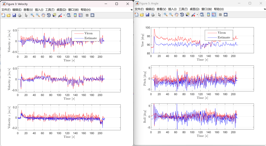
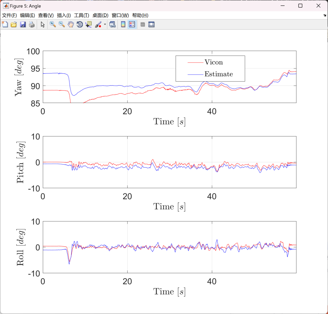
figure('name', 'Angle','position', [1278 100 840 630], 'color', [1 1 1]);
subplot(3, 1, 3);
plot(t, vcEul(1, :)*180/pi, 'r', t, px4Eul(1, :)*180/pi, 'b');
grid on;
ylim([-10, 10]);
set(gca, 'XTick',t(1):20:t(end));
xlabel('$\mathrm{Time}\ [s]$', 'interpreter', 'latex', 'fontsize', 14);
ylabel('$\mathrm{Roll}\ [deg]$', 'interpreter', 'latex', 'fontsize', 14);
set(gca, 'fontsize', 16);
subplot(3, 1, 2);
plot(t, vcEul(2, :)*180/pi, 'r', t, px4Eul(2, :)*180/pi, 'b');
grid on;
ylim([-10, 10]);
set(gca, 'XTick',t(1):20:t(end));
xlabel('$\mathrm{Time}\ [s]$', 'interpreter', 'latex', 'fontsize', 14);
ylabel('$\mathrm{Pitch}\ [deg]$', 'interpreter', 'latex', 'fontsize', 14);
set(gca, 'fontsize', 16);
subplot(3, 1, 1);
% plot(t, vcP(3, :), 'r', t, px4P(3, :), 'b', t, px4Lidar, 'g');
plot(t, vcEul(3, :)*180/pi, 'r', t, px4Eul(3, :)*180/pi, 'b');
grid on;
ylim([85, 100]);
set(gca, 'XTick',t(1):20:t(end));
xlabel('$\mathrm{Time}\ [s]$', 'interpreter', 'latex', 'fontsize', 14);
ylabel('$\mathrm{Yaw}\ [deg]$', 'interpreter', 'latex', 'fontsize', 14);
lghd = legend('$\mathrm{Vicon}$', '$\mathrm{Estimate}$');
set(lghd, 'interpreter', 'latex', 'fontsize', 14, 'position', [0.5360 0.8102 0.2117 0.1057]);
set(gca, 'fontsize', 16);
rmseyaw = rms(vcEul(3, :)*180/pi - px4Eul(3, :)*180/pi);
rmsepitch = rms(vcEul(2, :)*180/pi - px4Eul(2, :)*180/pi);
rmseroll = rms(vcEul(1, :)*180/pi - px4Eul(1, :)*180/pi);
stdyaw = std(vcEul(3, :)*180/pi - px4Eul(3, :)*180/pi);
stdpitch = std(vcEul(2, :)*180/pi - px4Eul(2, :)*180/pi);
stdroll = std(vcEul(1, :)*180/pi - px4Eul(1, :)*180/pi);
errsig = round([rmsex, rmsey, rmsez, maxTarVx, maxTarVy, maxTarVz;
stdx, stdy, stdz, 0, 0, 0], 3);
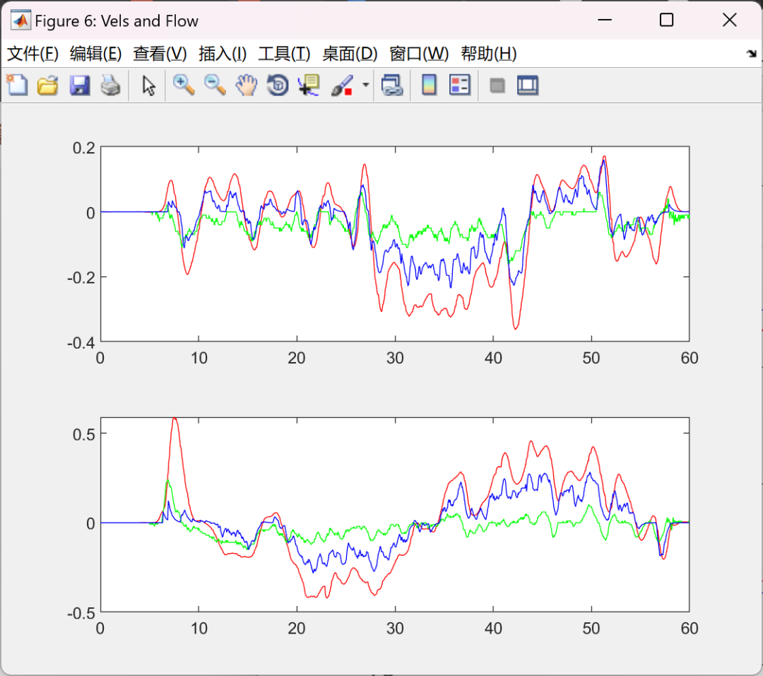
figure('name', 'Vels and Flow', 'position', [865 100 560 420]);
subplot(2, 1, 1);
plot(t, vcV(1, :), 'r', t, px4V(1, :), 'g', t, corflow(1, :).*vcP(3, :), 'b');
subplot(2, 1, 2);
plot(t, vcV(2, :), 'r', t, px4V(2, :), 'g', t, -corflow(2, :).*vcP(3, :), 'b');
03
References
03
References
Some content in this article is sourced from the internet, and references will be noted or cited as references. If there are any inaccuracies, please feel free to contact us for deletion. (The content of this article is for reference only, and specific effects are subject to the operating results)


04
Download MATLAB Code, Data, and Article
For more resources, follow us for MATLAB|Simulink|Python access