Python Data Analysis and Visualization
—— A Beginner’s Guide


To begin with, let me answer three fundamental questions to introduce you to the world of data analysis.
· Why Perform Data Analysis

We are in an era of information, where everything can be abstracted into information and data. To understand something, we need to understand its data information and the patterns of its data changes. In competitions, conducting data analysis appropriately helps in our decision-making and efficiency improvement.
· What is the Process of Data Analysis?

· Data Acquisition: Data is typically acquired using web scraping, databases, and file reading methods.
· Data Cleaning: The data we acquire is often not complete or flawless, and needs to undergo data type conversion and other processes before analysis.
· Data Analysis: This typically includes descriptive statistical analysis, visualization analysis, and cluster analysis.
· Conclusion Report: Write a conclusion analysis report that integrates data, analysis process, and conclusions.
· Why Choose Python?

Python is a high-level programming language with a simple syntax that is easy to learn. It also has a rich set of data analysis libraries such as NumPy, Pandas, and powerful visualization libraries such as Matplotlib and Seaborn. This gives it a significant advantage in the field of data analysis compared to other languages.

PART 1

Environment Setup

1►
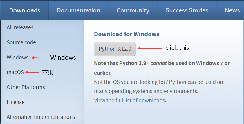
Download Python
Download the installation package directly from the official website and customize the installation location during installation. Official website:
https://www.python.org/
2►
Download Vscode and Python Extensions
Vscode is a powerful compiler, and its environment setup is relatively simple for beginners. Official website:
https://code.visualstudio.com/Download
After downloading, install the Python extension to compile Python programs. Besides the Python extension, I also recommend downloading the following extensions.
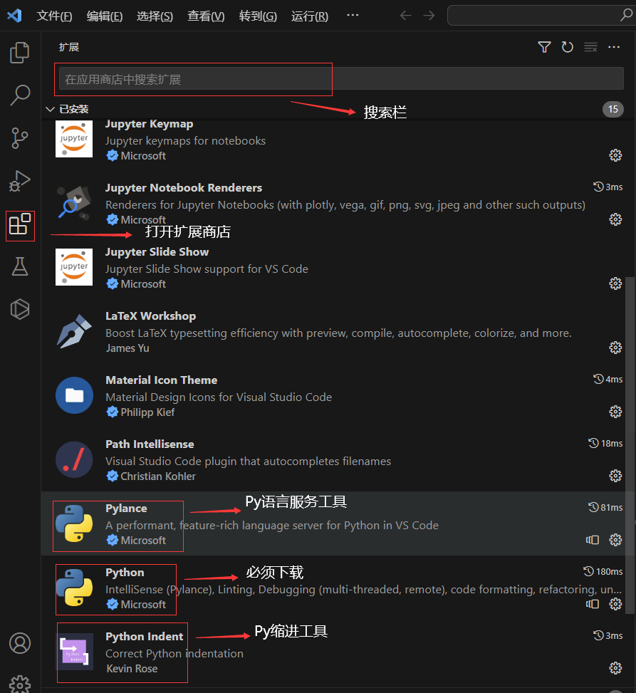
Students can also download Chinese localization extensions and other plugins they like as needed.
3►
Download Related Packages
This article uses three third-party libraries: NumPy, Pandas, and Matplotlib. I provide two download methods here.
· Install via pip
Open the command line tool with win+R, type cmd, and press enter to open the terminal. It is recommended to use Tsinghua mirror site for faster download speeds in China. Type the following code:
pip install numpy -i https://pypi.tuna.tsinghua.edu.cn/simplepip install matplotlib -i https://pypi.tuna.tsinghua.edu.cn/simplepip install pandas -i https://pypi.tuna.tsinghua.edu.cn/simpleSwipe left and right to view
· Download from the website
Open the mirror site:
https://pypi.tuna.tsinghua.edu.cn/simple/numpy/
Find the three libraries mentioned above and download them. After downloading, cut the three libraries into the Lib folder in the downloaded Python directory.
After downloading, verify by creating a new Python file in Vscode and typing:
import numpyimport pandasimport matplotlibIf there is no error, it means the installation was successful.


PART 2

Introduction to Numpy

1►
Introduction to NumPy
NumPy, short for Numerical Python, is an open-source numerical computing extension for Python. It is a Python library that provides multidimensional array objects, various derived objects (such as masked arrays and matrices), and various APIs for fast array operations.
The core of numpy lies in its array type, which, due to its underlying C language, allows array operations to be up to fifty times faster than Python’s list type. In data processing work, numpy is typically used for numerical calculations.
· Importing the NumPy Library
np is the conventional name for numpy.
import numpy as np· Query Functions
NumPy has many methods, and using the info() method allows for quick reference to the related documentation.
numpy.info(numyp.info) # Running will return documentation related to the numpy.info() functionSwipe left and right to view
2►
NumPy Data Types
To facilitate extensive calculations, numpy has set more data types than Python, for example, when a set of data is all less than 256, int8 can be used, which effectively reduces memory compared to Python’s built-in int (64-bit).
|
Data Type |
Description
Unique Identifier
bool
Boolean type stored in one byte
‘b’
int8
One byte size, -128 to 127
‘i1’
int16
Integer, 16-bit integer
‘i2’
uint8
Unsigned integer, 0 to 255
‘u1’
uint16
Unsigned integer, 0 to 65535
‘u2’
uint32
Unsigned integer, 0 to 2 ** 32 – 1
‘u4’
float16
Half-precision floating point: 16 bits, sign bit 1, exponent 5
‘f2’
float32
Single-precision floating point: 32 bits, sign bit 1, exponent 8
‘f4’
complex64
Complex number represented by two 32-bit floating point numbers for real and imaginary parts
‘c8’
complex128
Complex number represented by two 64-bit floating point numbers for real and imaginary parts
‘c16’
object
Python object
‘O’
string
String
‘S’
Swipe down to view
3►
Arrays
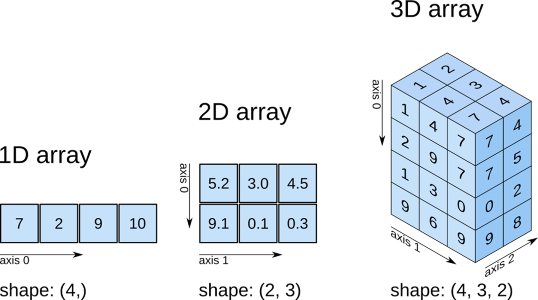
(Image source: Internet)
Unlike lists, arrays have a fixed size when created, and all elements in an array must have the same data type. Common types include one-dimensional arrays, two-dimensional arrays, and three-dimensional arrays.
The NumPy library uses axis to represent axes, specifying a certain axis means performing operations along that axis.
· Creating Arrays
· array() function
The simplest way to create an array is to pass in a list or tuple:
numpy.array(object, dtype=None, copy=True, order='K', subok=False, ndmin=0, like=None)Swipe left and right to view
Key parameter explanations:
|
Parameter |
Description |
|
object |
Any object exposing the array interface method |
|
dtype |
Data type |
|
copy |
If True, the object is copied; otherwise, a copy is only made if __array__ returns a copy, the object is a nested sequence, or a copy is needed to satisfy any other requirements (dtype, order, etc.). |
· arange() function
Creates an array with fixed step size by specifying the endpoints:
numpy.arange([start, ]stop, [step, ]dtype=None, *, like=None)Swipe left and right to view
Key parameter explanations:
|
Parameter |
Description |
|
start |
Starting value, default is 0 |
|
stop |
Ending value (not included) |
|
step |
Step size, default is 1 |
|
dtype |
Data type of the created ndarray, if not provided, the input data type will be used. |
· linspace() function
Creates an array by specifying the endpoints with a fixed number of elements:
numpy.linspace(start, stop, num=50, endpoint=True, retstep=False, dtype=None, axis=0)Swipe left and right to view
· logspace() function
Creates an array by specifying the endpoints with geometric progression:
numpy.logspace(start, stop, num=50, endpoint=True, retstep=False, dtype=None, axis=0)Swipe left and right to view
· empty() function
Creates an uninitialized array with specified shape (shape) and data type (dtype), with values generated randomly based on memory conditions:
numpy.empty(shape, dtype=float, order='C', *, like=None)Swipe left and right to view
· zeros() function
Creates an array filled with zeros of specified shape (shape) and data type (dtype):
numpy.zeros(shape, dtype=float, order='C', *, like=None)Swipe left and right to view
· full() function
Creates an array of specified shape and fills it with specified values:
numpy.full(shape, fill_value, dtype=None, order='C', *, like=None)Swipe left and right to view
· Basic Operations on Arrays
· Array Properties
Assuming we have an ndarray array, the important properties of the array are as follows:
|
Property |
Description |
|
ndarray.ndim |
Rank, i.e., the number of axes or dimensions |
|
ndarray.shape |
The dimensions of the array, for matrices, n rows m columns |
|
ndarray.size |
The total number of elements in the array, equivalent to the value of n*m in .shape |
|
ndarray.dtype |
The element type of the ndarray object |
|
ndarray.itemsize |
The size of each element in the ndarray object, in bytes |
|
ndarray.nbytes |
The total number of bytes consumed by the array elements |
|
ndarray.real |
The real part of the ndarray elements (real part of complex numbers) |
|
ndarray.imag |
The imaginary part of the ndarray elements (imaginary part of complex numbers) |
|
ndarray.T |
Transpose the array |
|
ndarray.flat |
A one-dimensional iterator over the array |
|
ndarray.flags |
Memory information of the ndarray object |
|
ndarray.strides |
Byte tuple for each dimension when traversing the array |
· Array Indexing and Slicing
Indexing and slicing of arrays in numpy is very flexible. Any array can be sliced in any way. An example is shown below:
import numpy as npa = np.arange(36).reshape(6, 6) # Generate a 6x6 two-dimensional arrayprint(a)Swipe left and right to view
The output is:
[[ 0 1 2 3 4 5] [ 6 7 8 9 10 11] [12 13 14 15 16 17] [18 19 20 21 22 23] [24 25 26 27 28 29] [30 31 32 33 34 35]]Slicing it:
print(a[3,0]) # Returns the element in the 4th row and 1st columnprint(a[1]) # Returns the 2nd rowprint(a[1,3:5]) # Returns columns 4 to 5 of the 2nd rowprint(a[4:,4:]) # Slices both the 5th row and columnprint(a[:,2]) # Returns the 3rd columnprint(a[2::2,::2]) # Slicing with a step of 2Swipe left and right to view
The output is:
18[ 6 7 8 9 10 11][ 9 10][[28 29] [34 35]][ 2 8 14 20 26 32][[12 14 16]55[24 26 28]]
tip
Unlike list slicing, the results of array slicing in NumPy are views of the array. Modifications to the view will affect the original array.
· Other Operations on Arrays
|
reshape() |
Used to reshape the array, i.e., change the shape of the array. The new shape must be compatible with the original shape, and the values in the array do not change. |
|
astype() |
This method is used to convert the types of elements in the array. It returns a new array with the original array’s values after type conversion, usually requiring only the type to convert to. |
|
copy() |
This method returns a copy of the specified array; modifications to the copy do not affect the original array. |
|
vstack() |
Vertically stacks arrays |
|
hstack() |
Horizontally stacks arrays |
|
vsplit() |
Splits the array by rows |
|
hsplit() |
Splits the array by columns |
|
delete() |
Used to delete specified rows or columns from the array and returns a new array after deletion. |
|
insert() |
Used to insert rows or columns at specified positions in the array and returns a new array after insertion. |
|
where() |
Queries elements that meet certain conditions |
|
sort() |
Sorts the array by value |
Swipe down to view
· Array Operations
When arrays a and b have the same shape, operations such as addition (+), subtraction (-), multiplication (*), division (/), exponentiation (**), integer division (//), and modulo (%) can be performed. Each element in the resulting array c corresponds to the result of the respective operation on the elements of arrays a and b.
Specifically, numpy supports matrix operations (@), as shown below:
import numpy as np
a = np.array([1,2,3,4]).reshape(2,2)b = np.array([1,0,2,1]).reshape(2,2)print(a @ b)
The output is:
[[ 5 2] [11 4]]

PART 3

Introduction to Pandas
1►
Pandas Overview
Pandas is an open-source library with a BSD license that provides high-performance, easy-to-use data structures and data analysis tools for the Python programming language. Compared to NumPy, Pandas is more convenient for data manipulation, while NumPy has an advantage in numerical calculations. Using both together often leads to better data analysis results.

· Importing the Pandas Library
pd is the conventional name for pandas.
import pandas as pd2►
Series and DataFrame
The pandas library provides two powerful data structure objects: Series and DataFrame. Mastering them can help simplify our data handling processes.
· Series
· Creating a Series
A Series is a one-dimensional labeled array, adding a label for indexing on top of the numpy array type. It can be created as follows:
pandas.Series(data=None, index=None, dtype=None, name=None, copy=False, fastpath=False)Swipe left and right to view
Parameter explanations:
|
data |
Data contained in the Series, supports lists, Numpy arrays, dictionaries, and scalar values |
|
index |
Row labels (indices) |
|
dtype |
Data type specified when the Series data is generated. If not specified, it will be inferred from the data automatically. |
|
name |
Specifies the index name |
|
copy |
Whether to copy data, default is False; in this case, it is a view, and modifications to the data in the Series will affect the data. |
The properties and operations of Series are similar to those of DataFrame, which will be introduced later.
· DataFrame
· Creating a DataFrame
pandas.DataFrame(data=None, index=None, columns=None, dtype=None, copy=None)Swipe left and right to view
A DataFrame is a two-dimensional labeled array, where the parameter meanings are the same as in the pandas.Series() method, with an additional parameter columns used to set column labels.
· DataFrame Properties
|
Method |
Function |
|
DataFrame.index |
Returns row labels |
|
DataFrame.columns |
Returns column labels |
|
DataFrame.dtypes |
Returns the data type of each column |
|
DataFrame.info() |
Views basic information about the DataFrame object, including index, data types, memory information, etc. |
|
DataFrame.values |
Returns the values of all elements |
|
DataFrame.size |
Returns the number of elements |
|
DataFrame.shape |
Returns the number of rows and columns of the DataFrame object |
· DataFrame Indexing and Slicing
The flexibility and versatility of indexing is what makes DataFrame powerful. Below, I will focus on introducing the iloc() and loc() indexing methods. Now we have a CSV file recording the number of students in the Mechatronics Innovation Team from 2020 to 2022, formatted as follows:
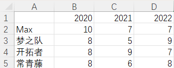
iloc(): Queries based on row and column index numbers, with index numbers starting from 0. Input can be: a single integer, a list or array of integers, or integer slices, as shown below:
import pandas as pddf = pd.read_csv('team_population.csv', index_col=0)print(df.iloc[0]) # Get a single row, returns the Max team population Seriesprint(df.iloc[[0, 1, 3]]) # Integer list to get multiple rows, returns Max, Dream Team, Ivy League populations DataFrameprint(df.iloc[0:2]) # Slice to get multiple rows, returns Max, Dream Team populations DataFrameprint(df.iloc[:, 1]) # Get a single column, returns the 21-level population of four teamsprint(df.iloc[:, [0, 2]]) # Integer list to get multiple columns, returns 20-level and 22-level team populations DataFrameprint(df.iloc[0:3, 0:2]) # Slice both row and column index, returns four teams' 20-level and 21-level populations DataFrameprint(df.iloc[0, 2]) # Row and column index, returns Max 22-level team populationSwipe left and right to view
The running result is as follows:
2020 102021 72022 7Name: Max, dtype: int64 2020 2021 2022Max 10 7 7Dream Team 8 5 9Ivy League 8 6 8 2020 2021 2022Max 10 7 7Dream Team 8 5 9Max 7Dream Team 5Pioneers 9Ivy League 6Name: 2021, dtype: int64 2020 2022Max 10 7Dream Team 8 9Pioneers 8 7Ivy League 8 8 2020 2021Max 10 7Dream Team 8 5Pioneers 8 97Swipe down to view
loc(): Queries based on row and column labels. Input can be: a single label, a list or array of labels, or label slices (with the slice including the end position), as shown below:
import pandas as pd
df = pd.read_csv('team_population.csv', index_col= 0)print(df.loc['Max'])                      # Get a single row, returns Max team population Seriesprint(df.loc[['Max','Dream Team','Ivy League']])     # Integer list to get multiple rows, returns Max, Dream Team, Ivy League populations DataFrameprint(df.loc['Max':'Pioneers'])             # Slice to get multiple rows, returns Max, Dream Team, Pioneers populations DataFrameprint(df.loc[:, '2021'])                  # Get a single column, returns the 21-level population of four teams Seriesprint(df.loc[:, ['2020', '2022']])        # Integer list to get multiple columns, returns 20-level and 22-level team populations DataFrameprint(df.loc['Max':'Ivy League', '2021':'2022'])      # Slice both row and column index, returns four teams' 21-level and 22-level populations DataFrameprint(df.loc['Max', '2022'])                               # Row and column index, returns Max 22-level team populationprint(df.loc['Max'].apply(lambda x:x>=7))           # Anonymous function filter, returns all Max team populations greater than or equal to 7 for the year
Swipe left and right to view
The running result is as follows:
2020 102021 72022 7Name: Max, dtype: int64 2020 2021 2022Max 10 7 7Dream Team 8 5 9Ivy League 8 6 8 2020 2021 2022Max 10 7 7Dream Team 8 5 9Max 7Dream Team 5Pioneers 9Ivy League 6Name: 2021, dtype: int64 2020 2022Max 10 7Dream Team 8 9Pioneers 8 7Ivy League 8 8 2021 2022Max 7 7Dream Team 5 9Pioneers 9 7Ivy League 6 872020 True2021 True2022 TrueName: Max, dtype: boolSwipe down to view
3►
Reading Files with Pandas
Pandas provides several flexible methods for reading files, which are simpler than Python’s native reading methods.
These include csv, json, excel, html, and many other commonly used file types. Below is a table summarizing these:
|
File Type |
Read |
Write |
|
CSV |
read_csv |
to_csv |
|
Fixed-Width Text File |
read_fwf |
– |
|
JSON |
read_json |
to_json |
|
HTML |
read_html |
to_html |
|
LaTeX |
– |
Styler.to_latex |
|
XML |
read_xml |
to_xml |
|
Local clipboard |
read_clipboard |
to_clipboard |
|
MS Excel |
read_excel |
to_excel |
|
OpenDocument |
read_excel |
– |
After reading, the function will return the corresponding series or DataFrame for further data analysis.
4►
Data Cleaning with Pandas
When the data we acquire is incomplete or has significant deviations, we need to perform preliminary cleaning to achieve better data analysis results.
The pandas library provides many methods for data cleaning.
· Handling Null and Missing Values
Pandas provides the isnull() and notnull() methods to check for missing values.
|
Function Name |
Function Effect |
|
isnull() |
Checks for null or missing values, returning a boolean value; returns True for missing values and False for non-missing values. |
|
notnull() |
Checks for null or missing values, returning a boolean value; returns False for missing values and True for non-missing values. |
· Handling Duplicate Values
For values that appear repeatedly in the data, pandas uses the duplicated() method for processing.
df.duplicated(subset=None, keep='first')Swipe left and right to view
Here, subset represents the column labels to check, and the function will return the corresponding boolean Series or DataFrame.
· Changing Data Types
When the data types in the data are inconsistent, we can use astype() to change the data types for convenience in subsequent calculations and analyses.
df.astype(dtype, copy=True, errors='raise')Swipe left and right to view
Here, dtype represents the data type to change to, and copy determines whether it is a copy.
· Resetting Index
When the original index does not align with our analysis goals, we can use the rename() method in pandas to rename the index.
df.rename(mapper=None, *, index=None, columns=None, axis=None, copy=True, inplace=False)Swipe left and right to view
Here, mapper, index, and columns are usually of dictionary type, with the original index as the key and the new index as the value.
· Data Transposition
Sometimes transposing the data can better meet our analysis needs. The stack() method in pandas can be used to stack columns into rows.
df.stack(level=- 1, dropna=True)Here, dropna indicates whether to drop missing values after transposition, default is True.
I have only listed a few commonly used data cleaning methods in the pandas library here; for more methods, you can refer to the official pandas documentation:
https://pypandas.cn/docs/


PART 4

Introduction to Matplotlib

1►
Overview of Matplotlib
Matplotlib is a Python 2D plotting library that generates publication-quality graphics in various hardcopy formats and interactive environments across platforms. The pyplot sub-library contains a set of command-style functions that make Matplotlib work similarly to MATLAB, significantly simplifying our function plotting tasks.

· Importing the pyplot Sub-library of Matplotlib
plt is the conventional name for pyplot.
import matplotlib.pyplot as plt2►
Plotting Operations
· plot() function
plt.plot(x, y)plot() is the most basic plotting method, where x and y are usually lists or arrays, and the image will be plotted with x as the horizontal coordinate and y as the vertical coordinate.
tip
If you want to use plot() to obtain a continuous smooth image, you can try using the linspace() function from the numpy library introduced earlier.
· show() function
plt.show()The show() function in the Matplotlib library is used to display images. Note that only the latest image will be retained in the background, so remember to use the show() function promptly after plotting.
· Image Decoration Functions
Matplotlib provides a rich set of image decoration functions. Below are some commonly used functions.
|
Function |
Description |
|
title() |
Adds a title to the current plot |
|
legend() |
Places a legend in the current plot |
|
annotate() |
Creates an annotation for specified data points |
|
xlabel(s) |
Sets the x-axis label |
|
ylabel(s) |
Sets the y-axis label |
|
xticks() |
Sets the positions and labels of x-axis ticks |
|
yticks() |
Sets the positions and labels of y-axis ticks |
This is just a very small part of the library; for more functions, you can learn from the official documentation.
3►
Plotting Examples
The Matplotlib library allows us to plot images with very concise code. Below are examples of several commonly used images.
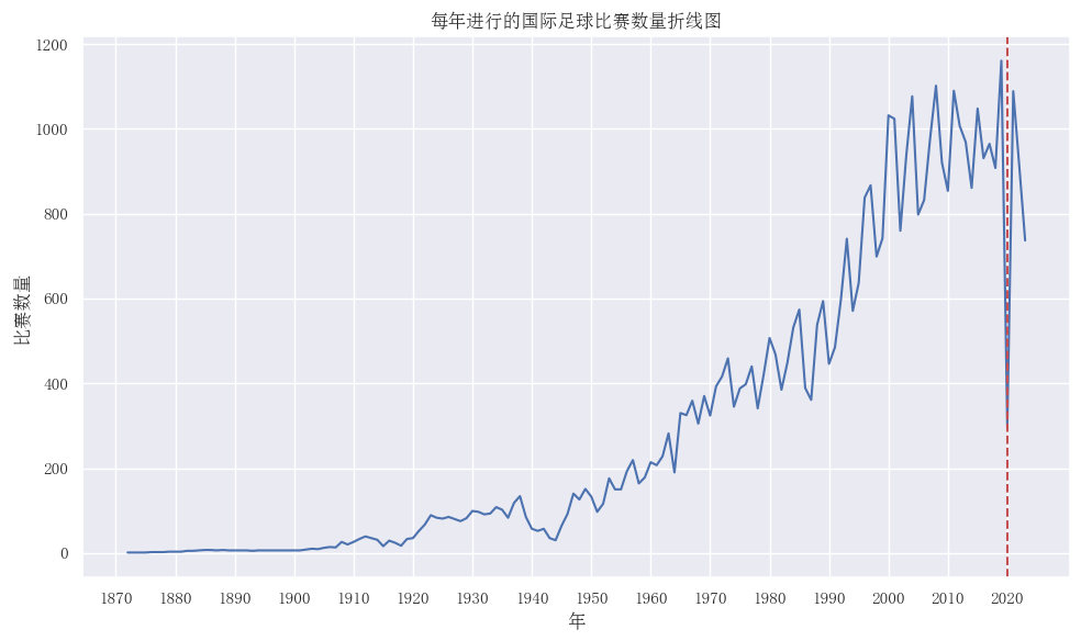
· Line Chart
Line charts are usually plotted using the plot() function. Below is a simple effect example.

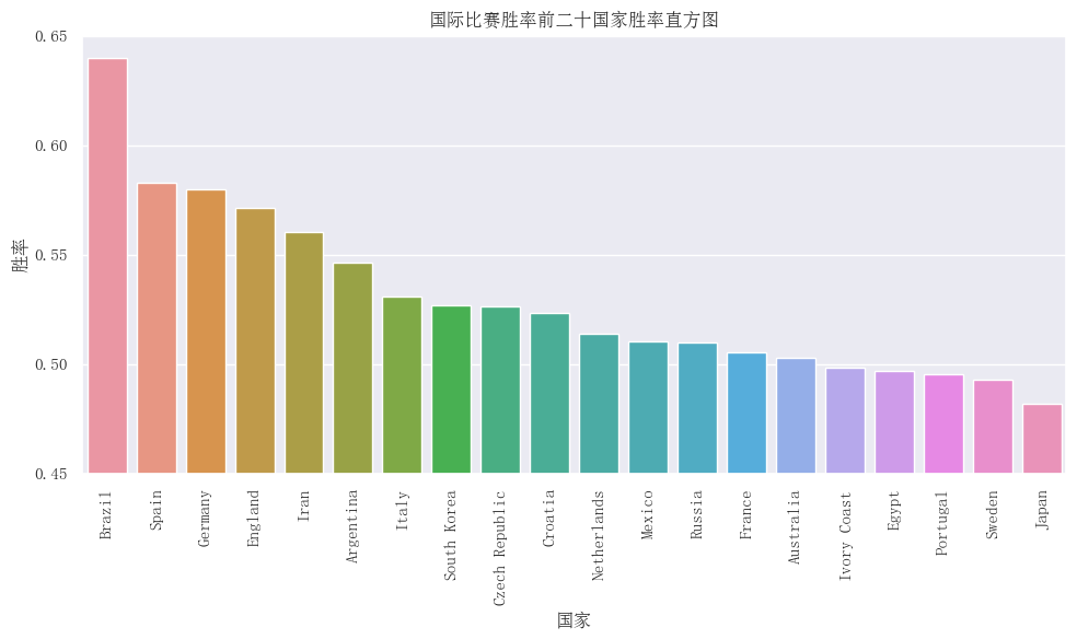
· Bar Chart
Bar charts are usually plotted using the bar() function, with a simple function prototype as follows:
plt.bar(x, height, width, bottom=None,color)Swipe left and right to view
Below is a simple effect example:
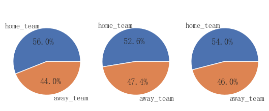
· Pie Chart
Pie charts are usually plotted using the pie() function, with a simple function prototype as follows:
pyplot.pie(x, explode=None, labels=None, colors=None)Swipe left and right to view
Below is a simple effect example:
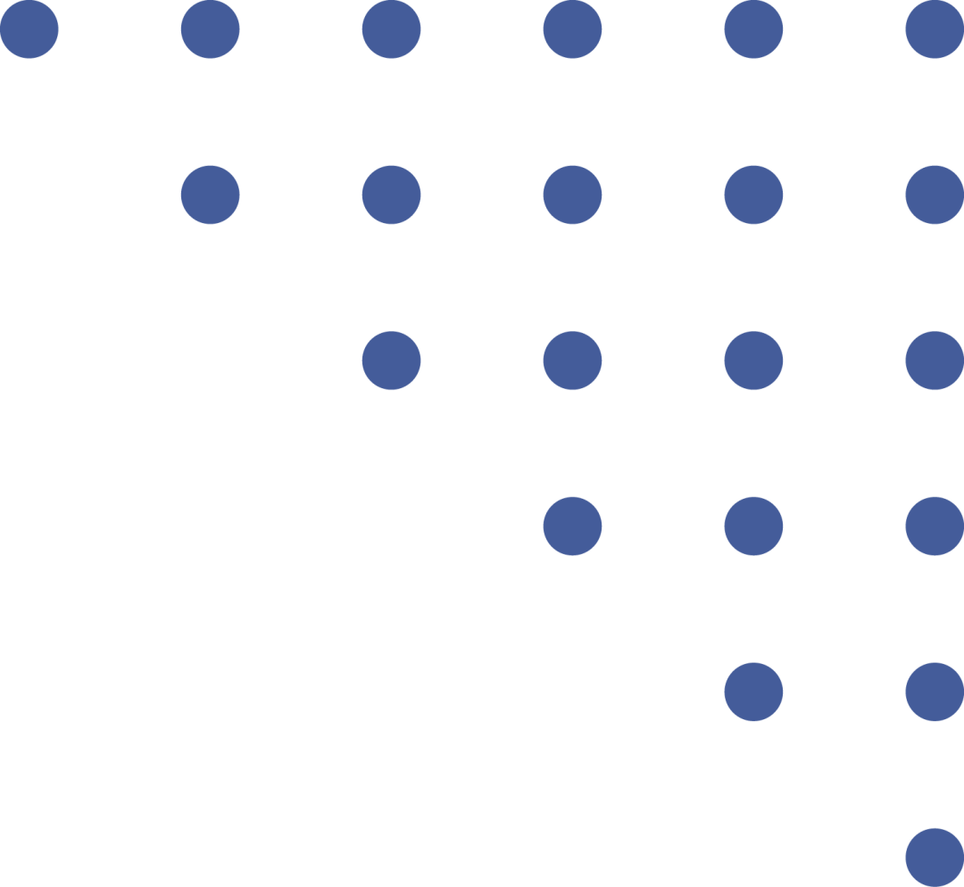
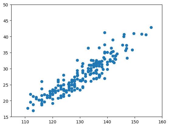
· Scatter Plot
Scatter plots are usually plotted using the scatter() function, with a simple function prototype as follows:
plt.scatter(x, y, s=None, c=None, marker=None)Swipe left and right to view
Below is a simple effect example:
The above is just a few of the most commonly used images; for more images such as radar charts and heat maps, you can refer to the official documentation of Matplotlib:
https://www.matplotlib.org.cn/API/


PART 5

Final Thoughts from the Author


In data analysis, I am also a beginner. The methods introduced in this article are the most basic applications among the libraries discussed. Python has a vast number of powerful data analysis libraries, and we need to frequently consult the official documentation and explore and experiment more to better understand the nuances of data analysis. Interested students can also continue learning about the sk-learn machine learning library and other tools to provide better fitting and more persuasive mathematical support for their analyses. I wish to progress together with everyone.
【End】

Scan to Follow Us

Text | Zhang Aoyu
Editor | Zhang Aoyu
Reviewer | Kou Yanlin Li Chenyang