
Click the top left corner to follow us

Gift to Readers
In the wonderful world of coding research, we can gain many unique insights. From the perspective of algorithm optimization, it is like carefully polishing a piece of art; each refinement of the code and improvement of the algorithm is akin to removing impurities, making it more efficient. This inspires us to continuously examine our ways of working in life and at work, seeking optimization opportunities to enhance efficiency. For example, when dealing with complex data, skillfully utilizing data structures and algorithms can transform originally chaotic information into an orderly format, reminding us to be adept at finding patterns and summarizing methods when faced with complex problems.
01/Overview
Introduction:
The Wireless Sensor Network (WSN), as a distributed monitoring system composed of numerous miniature sensor nodes, plays a crucial role in various fields such as environmental monitoring, military reconnaissance, smart agriculture, and industrial control. The reasonable layout of node locations directly affects the overall performance of the network, including coverage, connectivity, energy efficiency, and data transmission accuracy. Therefore, optimizing the locations of wireless sensor network nodes has become a core research topic for enhancing network performance, extending network lifespan, and meeting diverse application needs.
The Importance of Wireless Sensor Network Node Location Optimization
1. Coverage Optimization: Ensuring that sensor nodes can effectively cover the monitoring area, avoiding blind spots. For example, in forest fire monitoring, a reasonable node placement can comprehensively capture abnormal signals such as temperature and smoke in the forest, allowing for timely detection of fire hazards; in precision agriculture scenarios, accurately covering every corner of the farmland and monitoring soil moisture and nutrient content in real-time provides a basis for precise irrigation and fertilization.
2. Connectivity Assurance: Maintaining stable and reliable communication links between nodes to ensure smooth data transmission to the aggregation node. In urban intelligent traffic systems, sensor nodes deployed on various road segments can ensure real-time transmission of vehicle flow and speed data back to the control center through optimized location layouts, avoiding traffic information interruptions caused by node disconnections and ensuring normal system operation.
3. Energy Balancing: Optimizing node locations helps balance energy consumption among nodes in the network. Since sensor nodes typically rely on battery power, which is limited, if the layout is unreasonable, some nodes may exhaust their energy prematurely due to excessive data forwarding tasks, leading to network segmentation. A reasonable layout allows each node to share a relatively balanced workload, extending the overall lifespan of the network.
Goals and Constraints of Node Location Optimization
1. Objective Functions:Maximize Coverage Area: Expand the sensor nodes’ perception coverage of the monitoring area as much as possible to improve monitoring accuracy and comprehensiveness. For instance, in wildlife habitat monitoring, the goal is to capture every key area of animal activity. Minimize Energy Consumption: Aimed at extending network operating time, reducing unnecessary communication overhead between nodes, and lowering transmission power. For example, in environmental monitoring projects in remote areas, where battery replacement is difficult, energy-saving needs are particularly prominent. Enhance Network Connectivity: Ensure that nodes have sufficient connectivity to reduce transmission delays and packet loss rates. In monitoring networks for industrial automation production lines, it is crucial to ensure that production data is uploaded accurately and timely to avoid delays in production decision-making. Reduce Costs: Consider the costs of node deployment, maintenance, and subsequent operations comprehensively, reducing the number of nodes used or selecting low-cost sensor devices while meeting performance requirements. For example, in constructing large-scale smart home sensor networks, balancing user experience with cost investment is essential.
2. Constraints:Geographical Environment Limitations: The terrain, topography, and distribution of obstacles in the monitoring area restrict the placement of nodes. In geological disaster monitoring in mountainous areas, it is necessary to avoid dangerous areas such as cliffs and valleys where signals are easily obstructed; in urban environments with tall buildings, it is essential to consider the obstruction of signals by buildings and reasonably select locations such as between buildings or on rooftops. Node Energy Constraints: Each sensor node has a predetermined initial energy level, and its transmission distance and computing power are related to energy consumption. The layout must be planned according to energy budgets to prevent nodes from “dying” prematurely. Communication Radius Limitations: The wireless communication capability of nodes is limited, usually having a fixed communication radius. During optimization, it is necessary to ensure that adjacent nodes are within each other’s communication range to establish effective communication links. For example, in underwater sensor networks, the communication radius is significantly affected by signal attenuation in water, making it more limited.
Common Node Location Optimization Methods
1. Optimization Based on Deterministic Algorithms:Grid Division Method: The monitoring area is evenly divided into grids, and nodes are deployed at grid intersections or centers according to certain rules. For example, in regular farmland irrigation monitoring, soil moisture sensors can be placed at fixed intervals in a grid, which is simple and easy to implement, ensuring initial coverage uniformity. Geometric Shape-Based Methods: Utilize the characteristics of geometric shapes such as triangles and circles to plan node layouts. For instance, using an equilateral triangle layout in large flat areas for environmental monitoring can achieve high coverage efficiency and connectivity among nodes, with relatively balanced distances between nodes, facilitating energy management.
2. Optimization Based on Heuristic Algorithms:Genetic Algorithm: Simulates the biological evolution process, performing selection, crossover, and mutation operations on an initially randomly generated population of node positions, ultimately selecting the best node layout that meets optimization objectives after multiple generations of evolution. In complex terrain military monitoring scenarios, it can overcome uncertainties caused by geographical obstacles and find adaptive position combinations. Particle Swarm Optimization Algorithm: Treats node positions as particles in space, with particles dynamically adjusting their flight direction and speed based on their historical optimal positions and the group’s optimal position, ultimately converging near the optimal solution. In optimizing temperature and humidity monitoring networks for intelligent warehousing logistics, it can quickly adapt to changes in warehouse layouts and goods stacking, efficiently finding energy-saving and well-covered node positions. Simulated Annealing Algorithm: Based on the principle of metal annealing, it accepts inferior solutions with a certain probability to avoid falling into local optima, gradually reducing the temperature during the search process, transitioning from broad exploration to fine-tuning in the node position optimization process. In microenvironment monitoring for the protection of ancient buildings, it can effectively balance global search and local optimization, ensuring monitoring effectiveness.
Current Research Status and Challenges in Node Location Optimization
1. Research Status: Currently, significant achievements have been made in theoretical algorithm research for node location optimization, with various optimization algorithms continuously improved and integrated to enhance optimization effects. In practical applications, different fields customize optimization solutions based on their characteristics, such as in healthcare, where wearable sensor node positions are optimized to improve the accuracy of health data collection.
2. Challenges: Difficulty in Adapting to Dynamic Environments: Actual application scenarios are often subject to dynamic changes, such as temporary obstacles in the monitoring area, node failures, or new monitoring demands. Existing optimization methods struggle to adjust node positions in a timely and automatic manner to maintain stable network performance. Complex Trade-offs in Multi-Objective Optimization: When trying to meet multiple objectives such as coverage, connectivity, and energy efficiency, the objectives can constrain each other. Precisely determining objective weights and finding a comprehensive optimal solution remains a challenge. For example, in deploying sensor networks at emergency rescue sites, it is necessary to quickly and comprehensively cover the rescue area while considering the limited battery power of devices, making trade-offs challenging. Low Efficiency in Large-Scale Network Optimization: As the scale of sensor networks increases, with thousands of nodes or more, the computational complexity of traditional optimization algorithms rises sharply, leading to long computation times that fail to meet real-time requirements. For instance, in constructing large-scale infrastructure monitoring networks for smart cities, there is an urgent need for efficient optimization strategies.
02/Operating Results

03/Partial Code
close all
clear
clc
addpath(genpath(cd))
warnings('off')
%%
N=10; % number of nodes
area=[10,10]; % nodes deployment area in meter
Trange=2; % transmission range of sensor node in meter
nodes.pos=area(1).*rand(N,2);% nodes geographical locations
lambda=0.125; % signal wavelength in meter
nodes.major = Trange; % major axis for ellpitical range in meter
nodes.minor = lambda*Trange; % minro axis for ellipitical range in meter
% redundantNo=9; % number of healing nodes
redundantNo=round(10*N/100);
%% plot the nodes deployment
cnt=1;
for ii=1:N
for jj=1:N
if ii~=jj
nodes.distance(ii,jj)=pdist([nodes.pos(ii,:);nodes.pos(jj,:)]);
if nodes.distance(ii,jj)<Trange || nodes.distance(ii,jj)==Trange
nodes.inrange(ii,jj)=1;
else
nodes.inrange(ii,jj)=0;
end
end
end
end
figure
F5=plot(nodes.pos(:,1),nodes.pos(:,2),'.','color','r');
hold on
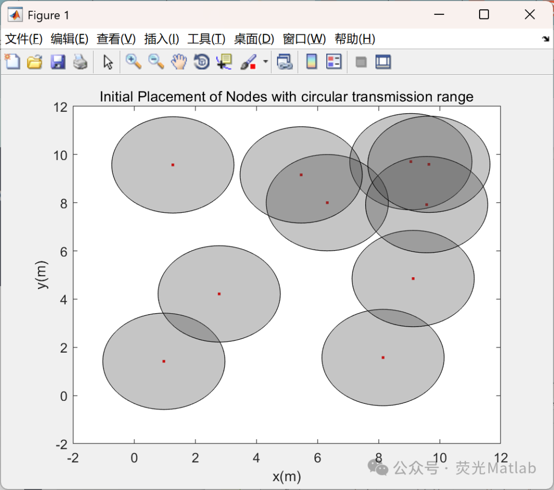
for ii=1:N % plot the circular transmission range
[nodes.circle.x(ii,:),nodes.circle.y(ii,:)]=circle(nodes.pos(ii,1),nodes.pos(ii,2),Trange);
F6=fill(nodes.circle.x(ii,:),nodes.circle.y(ii,:),[0.25,0.25,0.25]);
alpha 0.3
hold on
end
axis on
xlabel('x(m)')
ylabel('y(m)')
title('Initial Placement of Nodes with circular transmission range')
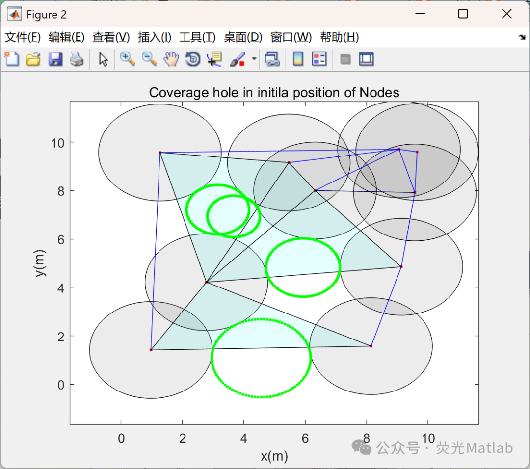
%% plot delauny triangle
TRI = delaunay(nodes.pos(:,1),nodes.pos(:,2));
figure(2)
F5 = plot(nodes.pos(:,1),nodes.pos(:,2),'.','color','r');
hold on
for ii=1:N % plot the circular transmission range
[nodes.circle.x(ii,:),nodes.circle.y(ii,:)]=circle(nodes.pos(ii,1),nodes.pos(ii,2),Trange);
F6=fill(nodes.circle.x(ii,:),nodes.circle.y(ii,:),[0.25,0.25,0.25]);
alpha 0.3
hold on
end
axis on
xlabel('x(m)')
ylabel('y(m)')
title('Coverage hole in initila position of Nodes')
hold on
triplot(TRI,nodes.pos(:,1),nodes.pos(:,2))
%% Hole detection
[holeDetected.circle,Circmcenter.circle,circumradius.circle]=holeDetection(TRI,nodes,F5,F6,Trange,area,2,1);
display(['--> No of detected Holes for Circular = ',num2str(numel(find(holeDetected.circle)))])
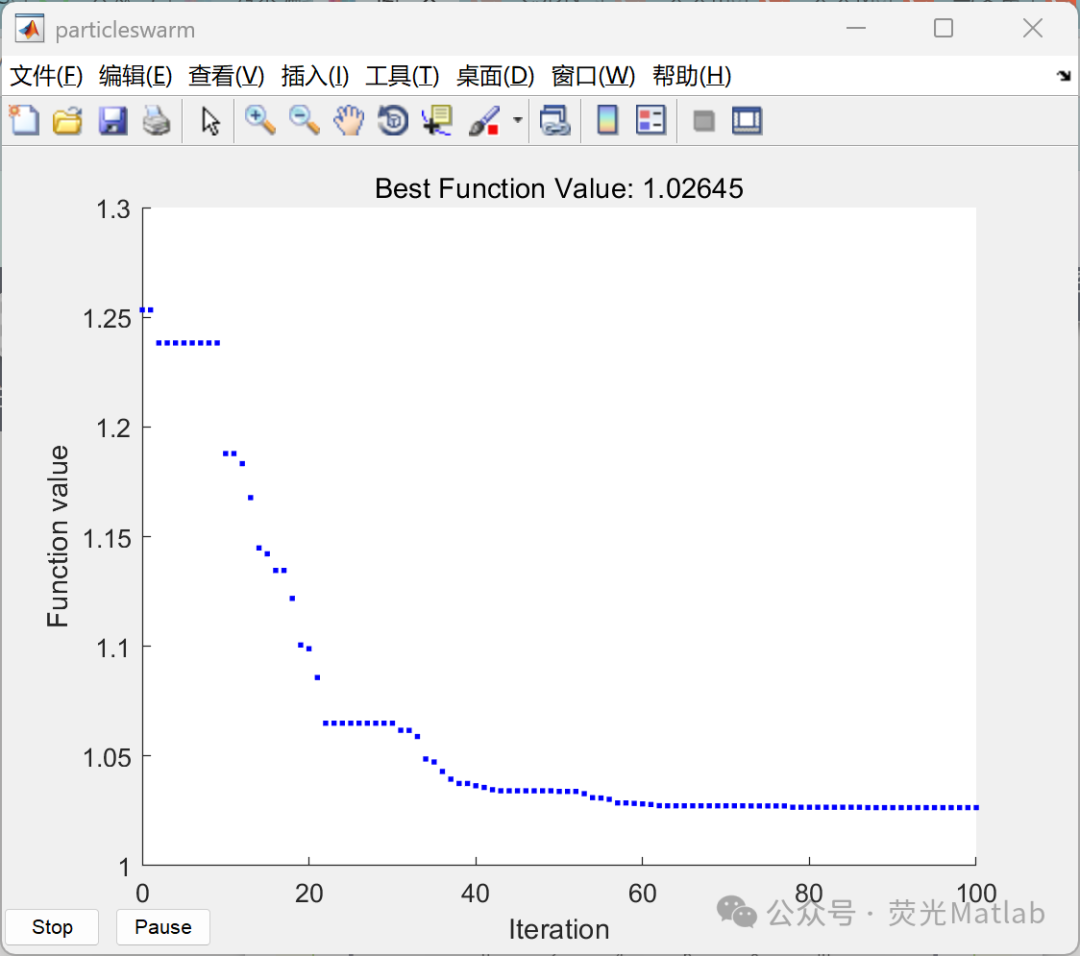
%% PSO optimize position of rest wsn nodes to cover the hole
nvars = 2*(N);
fun=@(x)objf(x,Trange,area);
lb=zeros(nvars,1);
ub=area(1).*ones(nvars,1);
options = optimoptions(@particleswarm,'Display','iter','MaxIterations',100,'PlotFcn','pswplotbestf');
[x,fval] = particleswarm(fun,nvars,lb,ub,options);
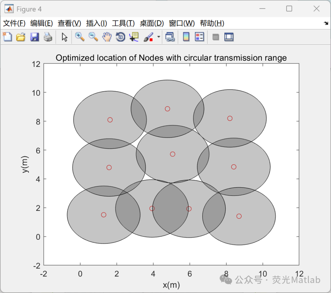
finalPos = reshape(x,[numel(x)/2,2]);
% plot the final tuned Node' pos
figure
plot(finalPos(:,1),finalPos(:,2),'o','color','r');
hold on
for ii=1:N % plot the circular transmission range
[finalcircle.x(ii,:),finalcircle.y(ii,:)]=circle(finalPos(ii,1),finalPos(ii,2),Trange);
fill(finalcircle.x(ii,:),finalcircle.y(ii,:),[0.25,0.25,0.25]);
alpha 0.3
hold on
end
04/References
[1] Jiang Zhanjun, Zhou Tao, Yang Yonghong. Privacy Strength Strategy for Optimizing Source Node Locations in Wireless Sensor Networks [J]. Progress in Laser and Optoelectronics, 2020, 57(24): 190-197.
[2] Miao Ruixin. Research on Coverage and Routing Optimization in Wireless Sensor Networks [D]. Changchun University of Science and Technology, 2020. DOI: 10.26977/d.cnki.gccgc.2020.000580.
Some content in this article is sourced from the internet, and references will be noted or cited as references. If there are any inaccuracies, please feel free to contact us for removal.


Scan to contact us!