Multi-task Learning and Beyond: Past, Present, and Future

Original text: https://zhuanlan.zhihu.com/

p/138597214

Author: Liu Shikun

Recently, there have been numerous breakthroughs in research on Multi-task Learning (MTL), along with many interesting new directions to explore. This has greatly inspired me to write a new article, attempting to summarize the recent research progress in MTL and explore future possibilities for other directions in MTL research.

This article will follow the general framework of my master’s thesis from 2018: Universal Representations: Towards Multi-Task Learning & Beyond, supplemented by recent methods from new articles and discussions on future directions.

Disclaimer: The articles mentioned in my master’s thesis were all preliminary results that were unpublished at the time. For anyone wanting to understand the details in the paper, please refer directly to the published conference articles.

Two Major Research Branches of Multi-task Learning

In most cases, MTL research can be categorized into the following two directions: one is MTL Network Design, and the other is MTL Loss Function Design. We will provide a detailed interpretation of these two directions below.

Multi-task Learning Network Design / What to Share? [Network Design]

Initially, MTL network design can typically be classified into two situations: Hard parameter sharing and Soft parameter sharing.

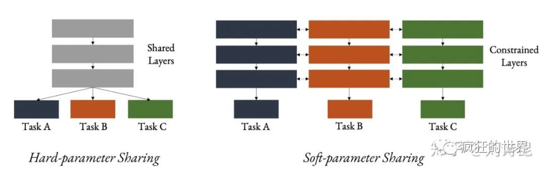
Hard-parameter sharing — is now almost an indispensable baseline for anyone doing MTL, where the entire backbone network is treated as a shared network to encode task information, and at the last layer, it splits into several task-specific decoders for prediction. Hard-parameter sharing serves as a lower bound (not strict, assuming no network pruning) for the parameter space of network design, thus serving as an important reference for evaluating new designs regarding the balance between efficiency and accuracy.

Soft-parameter sharing — can be seen as another extreme of hard-parameter sharing, and is not commonly found in current MTL network designs. In soft-parameter sharing, each task has its same-sized backbone network as the parameter space. We can impose specific constraints on this parameter space, such as sparsity, gradient similarity, or LASSO penalty, to softly constrain the representation space of different task networks. If we do not apply any constraints to the parameter space, soft-parameter sharing will collapse into single task learning.

Any MTL network design can be viewed as finding a balance point between hard and soft parameter sharing: 1. How to design the network to be compact and lightweight. 2. How to design the network to maximize the sharing of information among different tasks.

MTL network design is all about sharing.

• Cross-Stitch Network

The Cross-Stitch Network is a classic network design from the past few years and has been commonly used as a baseline in various MTL studies. Its core idea is to connect each independent task-specific network using learnable parameters (cross-stitch units) in a linear combination to link different tasks’ convolutional blocks.

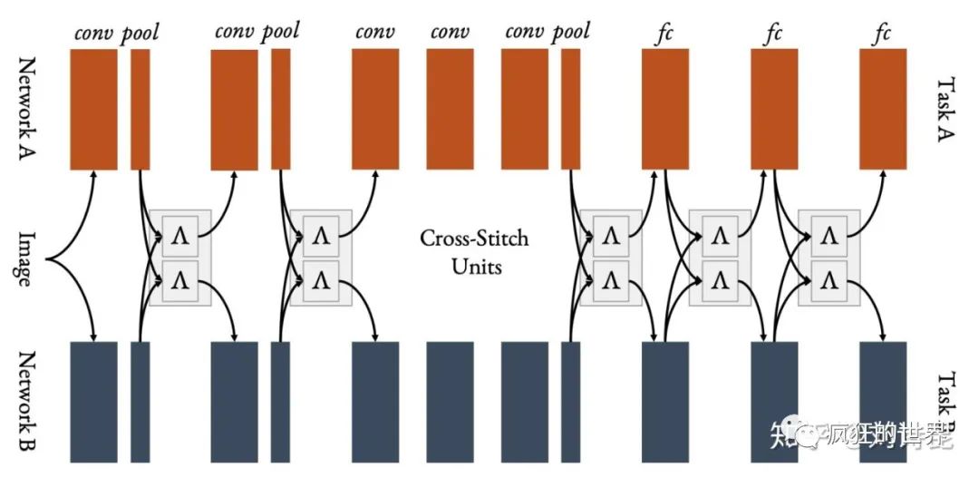
For tasks A and B, for each convolutional block output layer, we will calculate:

Through such operations, the input layer of the next convolutional block will be.

Inspired by the design of Cross-Stitch, NDDR-CNN also has a similar idea. However, unlike Cross-Stitch, they use concatenation and a [1 x 1] convolutional layer to reduce dimensionality for the information fusion of intermediate convolutional blocks. This design allows each task’s channel to intermingle information with channels of different indices, avoiding the limitation where the original Cross-Stitch could only infuse information from the same channel. When the non-diagonal elements of the convolutional layer weights in NDDR are 0, NDDR-CNN is mathematically equivalent to Cross-Stitch Network.

The major weakness of Cross-Stitch Network and NDDR-CNN is that a new network is required for each task, leading to a linear increase in the entire parameter space with the number of tasks, making it inefficient.

• Multi-task Attention Network

Based on the efficiency drawbacks of Cross-Stitch Network, I later proposed the Multi-task Attention Network (MTAN) to make the network design more compact, where the entire network’s parameter space increases sub-linearly with the number of tasks.

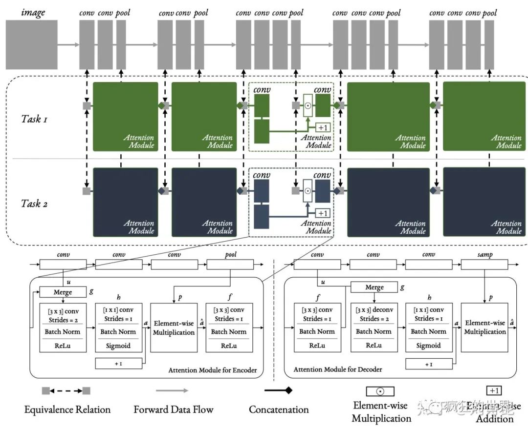
The core idea of MTAN is to assume that after the shared network encodes general representation information, we only need a small number of parameters to refine the task-shared representation into task-specific representation, which can yield a good representation for any task. Thus, the entire network only needs to add a small number of task-specific attention modules, two layers of [1 x 1] convolution layers, as additional parameter space to attend to the task-shared representation. The parameters of the entire model are significantly reduced compared to the Cross-Stitch Network.

• AdaShare

AdaShare takes the efficiency of MTL network design to the extreme. Instead of adding extra convolution layers to refine the task-shared representation, AdaShare treats a single backbone network as a whole representation, using a differentiable task-specific policy to decide whether to update or utilize the representation of a block of this network for any task.

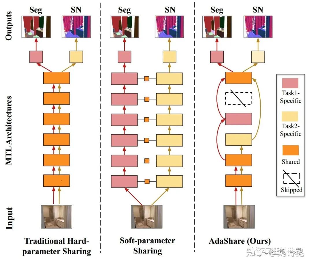
Since the entire network applies to the representation for all tasks, the network parameter space is agnostic to the number of tasks and remains constant, equivalent to hard-parameter sharing. The attached task-specific policy uses gumbel-softmax for each convolution block to categorical sample between two policies: “select” or “skip”. Thus, the design of the entire MTL network will change with different tasks, similar to the recently popular idea of Neural Architecture Search.

• MTL + NAS

MTL-NAS is another example that combines MTL and NAS. It builds on the core idea of NDDR, extending it to the fusion of arbitrary blocks, allowing the network to search for the best performance by merging different blocks of different tasks.

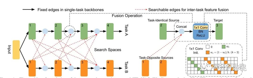
I personally prefer the search method of AdaShare, which searches layer by layer within a single network. This task-specific representation is already good enough compared to defining each task as a new network. Thus, MTL-NAS cannot escape the characteristic of linear increase in network parameters, but it provides new ideas for MTL network design.

MTL + NAS and traditional single-task NAS have different requirements and training methods.

1. MTL + NAS is not suitable for the most common two-stage training method in NAS: using validation performance as supervision to update architecture parameters, obtaining a converged architecture, and then re-training the entire network. Because the fused information in MTL has a training-adaptive nature, fixing the network structure will lead to the loss of this training-adaptive information, resulting in performance lower than the one-stage approach that searches and converges simultaneously. In other words, oscillation during training and feature fusion is more important for MTL networks, whereas there is no concept of feature fusion in single task learning. This indirectly leads to different demands for NAS training methods.

2. MTL + NAS is task-specific. In NAS training, if the dataset’s complexity is too high, we sometimes use proxy tasks to speed up training. The most common case is using CIFAR-10 as a proxy dataset to search for good network structures to be applied to the larger ImageNet dataset. However, this method is not applicable to MTL because the feature information and task characteristics required for any task or pairs of tasks are not the same, making it impossible to accelerate training through proxy tasks. Each task’s network is unique and distinct.

I believe that in future research on MTL network design, we will achieve more interpretable and human-understandable network characteristics, allowing us to understand the relationships and complexities between tasks. Through the obtained task correlations, we can use them as good prior knowledge to initialize a better starting network, thereby resulting in a superior model and a positive feedback loop.

A Better Task Relationship A Better Multi-task Architecture

Multi-task Learning Loss Function Design / How to Learn? [Loss Function Design and Gradient Optimization]

Parallel to network design, another popular direction is the design of MTL loss functions, or understanding how to better update the task-specific gradients in the network.

For any task i, we have the loss function: , where are the task-specific learning parameters. We need to find a good set to optimize the performance of all tasks i. The simplest and most direct way is equal weighting: , which assumes that each task contributes equally to the representation.

• Weight Uncertainty

Weight Uncertainty is one of the earliest studies on MTL loss function design. This article assumes that there is a data-agnostic task-dependent uncertainty in each model called Homoscedastic uncertainty (this term is quite peculiar and is mainly used by the Cambridge group). By maximizing the log-likelihood of the model prediction uncertainty, we can balance MTL training. Here, the likelihood (usually parameterized by Gaussian) can be seen as the relative confidence between tasks.

For any model prediction y, we define the Gaussian likelihood of the model: where here is the learnable noise scalar (Gaussian variance), and we need to maximize:

,

Thus, we can derive a newly defined loss function:

.

The final derived formula is very concise, and thus it has been used in many MTL benchmarks.

However, this article has sparked considerable controversy, particularly because the author has persistently refused to open-source such a simple formula and has ignored numerous inquiries from other researchers regarding implementation details, angering many peers (including myself). Furthermore, weight uncertainty is highly dependent on the choice of optimizer; in my personal experiments, I found that only the ADAM optimizer allows weight uncertainty to converge correctly, while no convergence trend was observed with other optimizers. This blog points out that this weight uncertainty formula can directly lead to a closed-form solution: when the learnable is minimized, the entire loss function will transform into the geometric mean of task losses, thus raising questions about the feasibility of this uncertainty assumption.

• GradNorm

GradNorm is another early work on MTL loss function. The implementation of GradNorm balances the gradient updates between different tasks by calculating the inverse training rate: the rate of descent, as an indicator.

We define W as the L2-norm of the weighted multi-task loss at time step t; the mean task gradient is; relative inverse training rate is . GradNorm updates task-specific weighting through the following objective:

where is the ideal gradient L2-norm (as a constant) to adjust task-specific weighting. As a balancing hyperparameter, the larger it is, the more balanced the task-specific weighting becomes. Since each calculation requires backpropagation through all tasks at each layer, it is computationally expensive. Thus, the author approximates by calculating the shared layer of the last layer to speed up training.

• Dynamic Weight Average

Since GradNorm requires two backpropagation calculations to compute task-specific weighting, it is very complex in implementation. I later proposed a simpler method that calculates task weighting only by computing the relative descending rate of loss:

Here, the is calculated by the loss ratio of two adjacent time steps as the descending rate. Therefore, the smaller it is, the greater the convergence rate, the simpler the task, and the smaller the obtained weight.

• MTL as Multi-objective Optimization

Several task-weighting methods introduced earlier are based on specific heuristics, making it difficult to guarantee optimum in MTL optimization. In MTL as Multi-objective Optimization, the authors view the MTL problem as a multi-objective optimization problem, aiming to achieve Pareto optimum.

Pareto optimum refers to any improvement in the performance of one task will necessarily lead to a decline in the performance of all remaining tasks. The authors utilize a method called multiple gradient descent algorithm (MGDA) to find this Pareto stationary point. The general approach is that after calculating task-specific gradients each time, it obtains a common direction to update shared parameters. If this common direction exists, the entire optimization has not yet converged to the Pareto optimum. This convergence method ensures that shared parameters do not experience conflicting gradients, allowing each task’s loss to converge more smoothly.

• Other Heuristic Methods

In the design of MTL loss functions, there are various other heuristic methods, either based on the difficulty of tasks (Dynamic Task Prioritization) or directly mapping the calculated task gradients to prevent conflicting gradients among tasks (Gradient Surgery).

However, among the various MTL loss function designs, it is rare for one method to outperform others across all datasets. In fact, in some datasets, the simplest equal task weighting also performs quite well. On one hand, the effectiveness of task weighting heavily depends on the design of the MTL network itself; furthermore, the updating of task weighting also depends on the dataset and optimizer. If the core goal is merely to achieve the best MTL performance, I would recommend spending more time researching better networks rather than task weighting. However, it cannot be denied that research on task weighting can better help people understand the correlations and complexities between tasks, which in turn assists in designing the model itself.

Auxiliary Learning — Not All Tasks Are Created Equal [Auxiliary Learning]

A highly related direction to MTL is called Auxiliary Learning (AL): its training process is entirely consistent with MTL. The only difference is that in Auxiliary Learning, only the performance of some tasks needs to be considered (primary task), while other (auxiliary) tasks exist to help the primary tasks learn better representations.

• Supervised Auxiliary Learning

Auxiliary Learning is more universal than we can imagine. For example, MTL is actually a special form of AL; we can treat any task in it as a primary task and the remaining tasks as auxiliary tasks. In MTL, we assume that all tasks have a mutually beneficial relationship, so all learning tasks benefit from this correlation.

Auxiliary Learning is also applied in many fields; for instance, this article found that training depth and normal prediction simultaneously can effectively help improve object detection accuracy. Or this article found that when reconstructing short sequences, it can help RNN train very long sequences more effectively.

In the setting of supervised auxiliary learning, the choice of the entire network and tasks heavily relies on human prior knowledge and does not possess absolute universality.

• Meta Auxiliary Learning

Considering the limitations of supervised auxiliary learning in task selection, I later proposed a meta-learning-based method to automatically generate auxiliary tasks, which I call Meta Auxiliary Learning (MAXL).

In traditional supervised auxiliary learning, I found the following two rules:

1. If the primary and auxiliary tasks are in the same domain, the performance of the primary task will improve only if the complexity of the auxiliary task is higher than that of the primary task.

2. If the primary and auxiliary tasks are in the same domain, the final performance of the primary task depends only on the complexity of the highest auxiliary task.

The definition of task complexity here is tricky and not general; currently, I only consider the simplest case of image classification: the complexity of fine classification tasks is higher than that of coarse classification tasks.

For example, in the figure below, we see the classification information for cats and dogs, which intuitively is lower than that of fine classification, such as Yorkshire, Persian cats, etc. The information required to classify cats and dogs is a subset of the information required to classify fine categories, leading to rule 2.

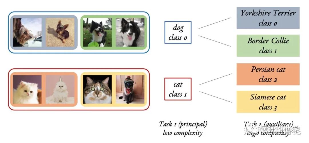
Given rule 2, we only need to consider the situation of training two simple tasks: one primary task and one auxiliary task. Therefore, the problem of “generating” a good auxiliary task can be transformed into generating good fine classification labels for any input image using a good network.

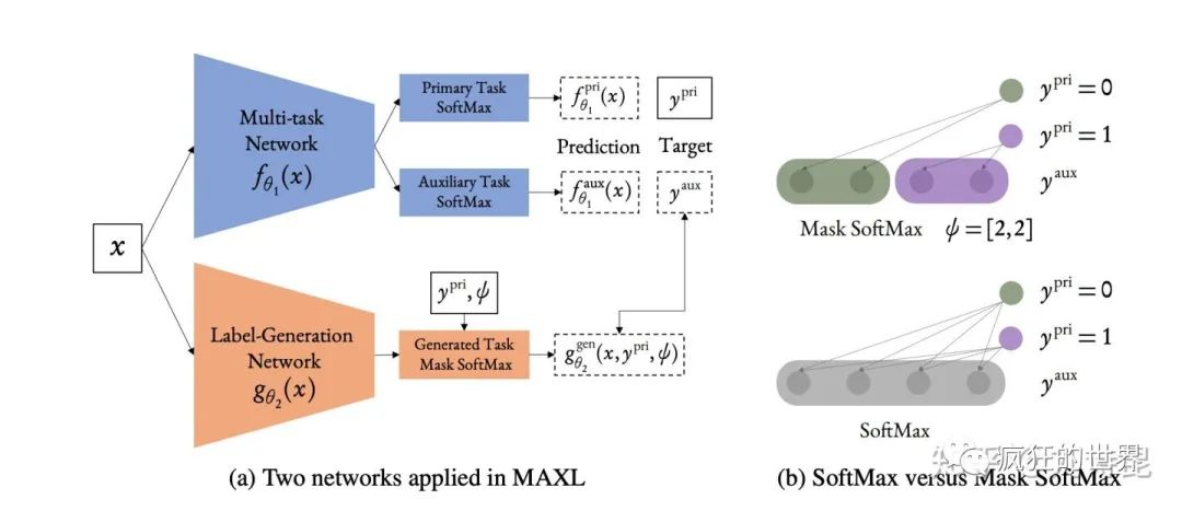
In the MAXL framework, we have two networks: one network is a multi-task network similar to hard parameter sharing to perform multi-task training. The other network is a label-generation network to generate fine classification labels, providing predictions for the multi-task network as auxiliary task labels.

Thus, for the Multi-task network, we need to make the following updates:

For the label-generation network, we need to perform the following updates through meta-update:

Where,

represents the meta-update, aiming to maximize the validation performance of the primary task to find the best auxiliary label. The second derivative trick here is akin to the gradient update in the classic meta-learning algorithm MAML.

In the label-generation network, there is also a hyper-parameter representing the human-defined dataset hierarchy. Suppose we are doing simple binary classification, then means further dividing the first class into 2 classes and the second class into 3 classes. The label-generation network generates corresponding suitable auxiliary labels through this hierarchy using a masked version of softmax. Thus, the multi-task network performs two classification tasks: the primary task is binary classification, and the auxiliary task is five-class classification.

Through MAXL, we found that it can improve performance for such image classification tasks. We later visualized the generated labels and found that in some simple datasets, they have human-understandable clustering significance.

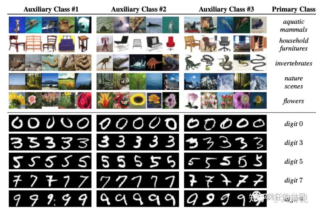
In the above image, the upper part shows the classification of CIFAR-100, while the lower part shows the classification of MNIST. Among these three auxiliary classes, the images are generated by the label-generation network, showing the five images with the highest confidence in that class.

In the more complex CIFAR-100 dataset, it is difficult to understand what MAXL’s classification is doing. However, in MNIST, we can see different thicknesses of the digit 3, different orientations of the digit 9, and digits 7 with or without a horizontal bar clustering together. This interesting phenomenon opens up a novel direction for exploring automated auxiliary task generation.

• Self-supervised Auxiliary Learning: Learning to X by Y

Auxiliary learning can also be applied in self-supervised learning, assuming that there are no human labels for either the primary task or the auxiliary task. The self-supervised training here, like supervised auxiliary tasks, effectively utilizes human prior knowledge regarding the characteristics of certain task combinations.

Common combinations include: depth and ego-motion predictions, which can maintain temporal consistency. Similarly, colorization and tracking, feature learning and ego-motion can also utilize such temporal consistency.

Such consistency can also exist in RL-based robot learning, such as grasping and pushing, or robot manipulation.

Conclusion

Finally, we come to the conclusion! In recent years, there have been many novel and valuable works in MTL research, but there is still significant room for improvement and understanding regarding the tasks themselves and the relationships between tasks. In Taskonomy, the authors attempted to create a relationship map among thousands of (massive CO2 emissions) tasks. However, in real MTL training, I believe this relationship map should change over time and depend on the network itself. Therefore, how to better optimize the network structure through task relationships remains an unsolved mystery, and how to design/generate auxiliary tasks to better assist the primary task is also not thoroughly understood. I hope to see more in-depth explorations of MTL in future research, achieving the ultimate vision of universal representation.

Important! The Yizhen Natural Language Processing - Pytorch group has been established. We have organized the official Pytorch Chinese version tutorial, add the assistant to receive it, and you can also enter the official group! Note: Please modify the remark to [School/Company + Name + Direction] when adding. For example - Harbin Institute of Technology + Zhang San + Dialogue System. The account owner, please consciously bypass. Thank you!

Recommended reading: NLP Learning (1) - Introduction to NER

NLP Learning (2) - Overview of NER

Softmax function and cross-entropy