Implementation of Nonlinear Fitting Methods in MATLAB

Source: This article is from Wang Fuchang’s blog on ScienceNet, Author: Wang Fuchang.

In MATLAB, there are commands for fitting such as polyfit, lsqcurvefit, nlinfit, and the curve fitting tool cftool, which are sufficient to solve general engineering fitting problems. Below are several commonly used functions.

p=polyfit(x,y,n) performs polynomial fitting on the data, obtaining the polynomial coefficients p, arranged in descending order, where the parameters x and y are vectors composed of data (xi,yi)(i=1,2,⋯,n), and n is the degree of the polynomial. For example:

x=[1, 3, 4, 6, 7];
y = [-2.1,-0.9,-0.6, 0.6, 0.9];
p = polyfit(x,y,1)

Thus, the fitting equation is:

Polynomial fitting can be transformed into a linear fitting problem, but most nonlinear fitting problems cannot be converted into linear fitting problems and require direct use of nonlinear least squares algorithms. Below are several methods.

The lsqnonlin() function solves nonlinear least squares problems.

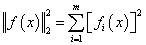
The usage format is:

[x, resnorm, residual, exitflag, output, lambda, jacobian] = lsqnonlin(fun,x0,lb,ub,options)

where fun is a vector function; x0 is the initial point; lb and ub are the lower and upper bounds of the variables, respectively; options are parameter options set by the optimset function. The variable x is the local minimum of the nonlinear least squares problem; resnorm is the sum of squares of residuals at x; residual is the residual value at x; exitflag is the exit condition; output is the output solving information; lambda is the Lagrange multiplier for the lower and upper bounds; Jacobian is the Jacobian matrix at x.

For example, to solve a nonlinear system of equations:

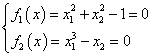
Set the initial point:

>> equs = @(x)[x(1)^2+x(2)^2-1; x(1)^3-x(2)];
x0 = [-0.8;0.6];
[x, resnorm, residual, exitflag, output, lambda, jacobian] = lsqnonlin(equs,x0)

The lsqcurvefit() function is a nonlinear least squares fitting function, with the usage format:

[x, resnorm, residual, exitflag, output, lambda, jacobian] = lsqcurvefit(fun,x0,xdata,ydata,lb,ub,options)

where fun is a vector function; x0 is the initial point; xdata and ydata are the fitting points; lb and ub are the lower and upper bounds of the variables, respectively; options are parameter options set by the optimset function. The variable x is the local minimum of the nonlinear least squares problem; resnorm is the sum of squares of residuals at x; residual is the residual value at x; exitflag is the exit condition; output is the output solving information; lambda is the Lagrange multiplier for the lower and upper bounds; Jacobian is the Jacobian matrix at x.

For example, given data:

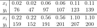
that satisfies the Michaelis-Menten equation:

to find parameters p₁ and p₂.

xdata = [0.02, 0.02,0.06,0.06,0.11 ,0.11,0.22,0.22,0.56,0.56,1.10,1.10];
ydata = [76, 47,97,107,123,139,159,152,191,201,207,200];
fun = @(p,xdata)(p(1)*xdata./(p(2)+xdata));
x0 = [200;0.1];
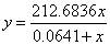
p = lsqcurvefit(fun,x0,xdata,ydata)

After running, we obtain:

Thus, the fitting function is:

The nlinfit() function is a nonlinear regression function, with the usage format:

[beta,r,J,Sigma,mse] = nlinfit(X,y,fun,beta0)

where parameter X is the design matrix; y is the response variable; fun is the regression (fitting) function; beta0 is the initial parameters; beta is the optimal regression parameters; r is the residual; J is the Jacobian matrix; SIGMA is the covariance matrix of the parameters; mse is the mean square error.

For example, given data:

that satisfies the Michaelis-Menten equation:

to find parameters p₁ and p₂.

x = [0.02, 0.02,0.06,0.06,0.11 ,0.11,0.22,0.22,0.56,0.56,1.10,1.10];
y   = [76, 47,97,107,123,139,159,152,191,201,207,200];
fun = @(beta,x)(beta(1)*x./(beta(2)+x));
beta0 = [200;0.1];
beta = nlinfit(x,y,fun,beta0)

Thus, the fitting function is:

In the lower right corner, please clickto like+👍

The editor’s salary will increase by 0.2 yuan

Free access: 600+ quality public courses totaling over 600 video courses, with a total duration of over 1000 hours

👇 Click to receive 👇