
Share interest, spread happiness,
increase knowledge, and leave beautiful.
Dear, this is the LearningYard Academy!
Today, the editor brings the
“Hui Xue (19): Learning to create inset plots in MATLAB”
Welcome to visit!
1. Mind Mapping
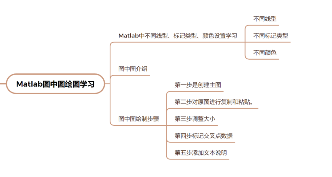
2. Learning to set different line styles, marker types, and colors in MATLAB
1. Different line styles
In MATLAB plotting, the line style determines the pattern of the connecting lines between data points on the graph. Common line styles include solid lines, dashed lines, dotted lines, etc. For example, entering ‘–‘ will connect the data points represented by x and y with dashed lines.

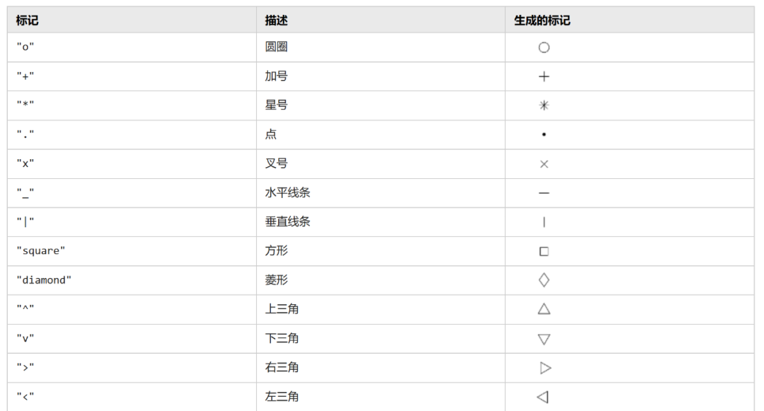
2. Different marker types
Markers are small symbols added at each data point to highlight their positions on the graph or to emphasize discrete points. For example, using ‘o’ will draw a circle at the location of each point, helping us see each data point more clearly.
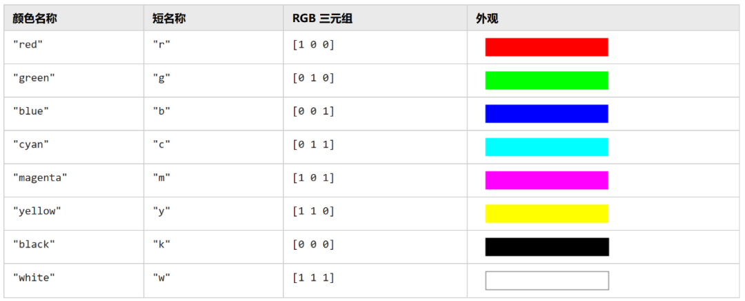
3. Different colors
In MATLAB, the color of a line can be represented by simple letters for common colors, such as ‘r’ for red and ‘b’ for blue. If you want to use more specific colors, you can also set the color using a vector with three numbers, known as an RGB triplet, which represents the intensities of red, green, and blue.
3. Introduction with inset plots
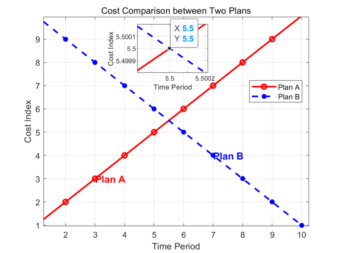
A “figure within a figure” embeds a smaller graph in a larger one to highlight local details (e.g., fluctuations, outliers) or compare data subsets. It enhances readability by magnifying key areas or contrasting methods/models. In MATLAB, this is done by duplicating or manually adding extra coordinate axes, not via a dedicated graph type.
4. The steps for drawing an inset plot
1. The first step is to create the main figure, where we can use the plot function to draw the primary data.
2. The second step involves using arrows to select the original figure, then right-clicking the mouse or directly using shortcut keys to copy and paste it.
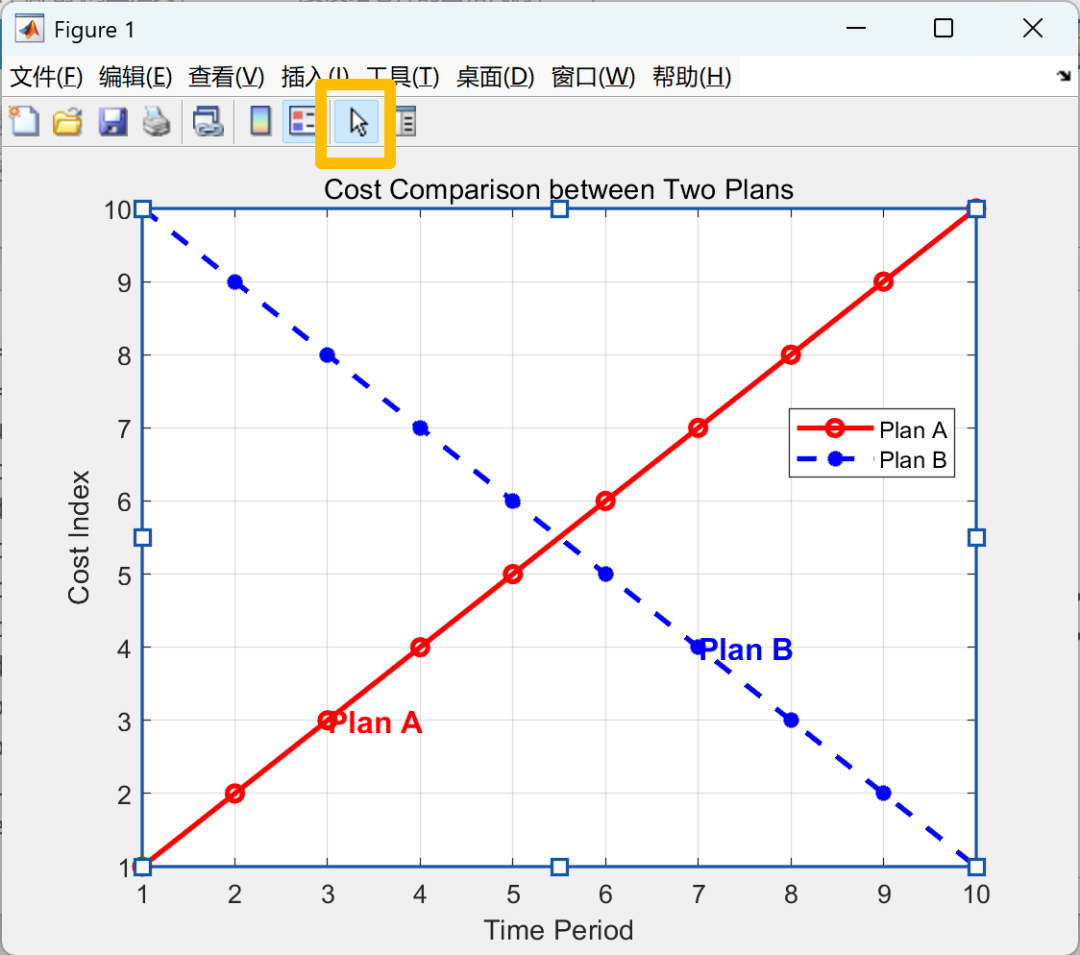
3. The third step is, after pasting the original figure, we can first resize the pasted image to an appropriate scale and move it to the desired position. Then, by clicking on the zoom-in, zoom-out, or pan tools in the toolbar and hovering the arrow over the pasted figure, we can directly see the display bars for these three tools and use them to adjust and highlight the area we want to magnify.
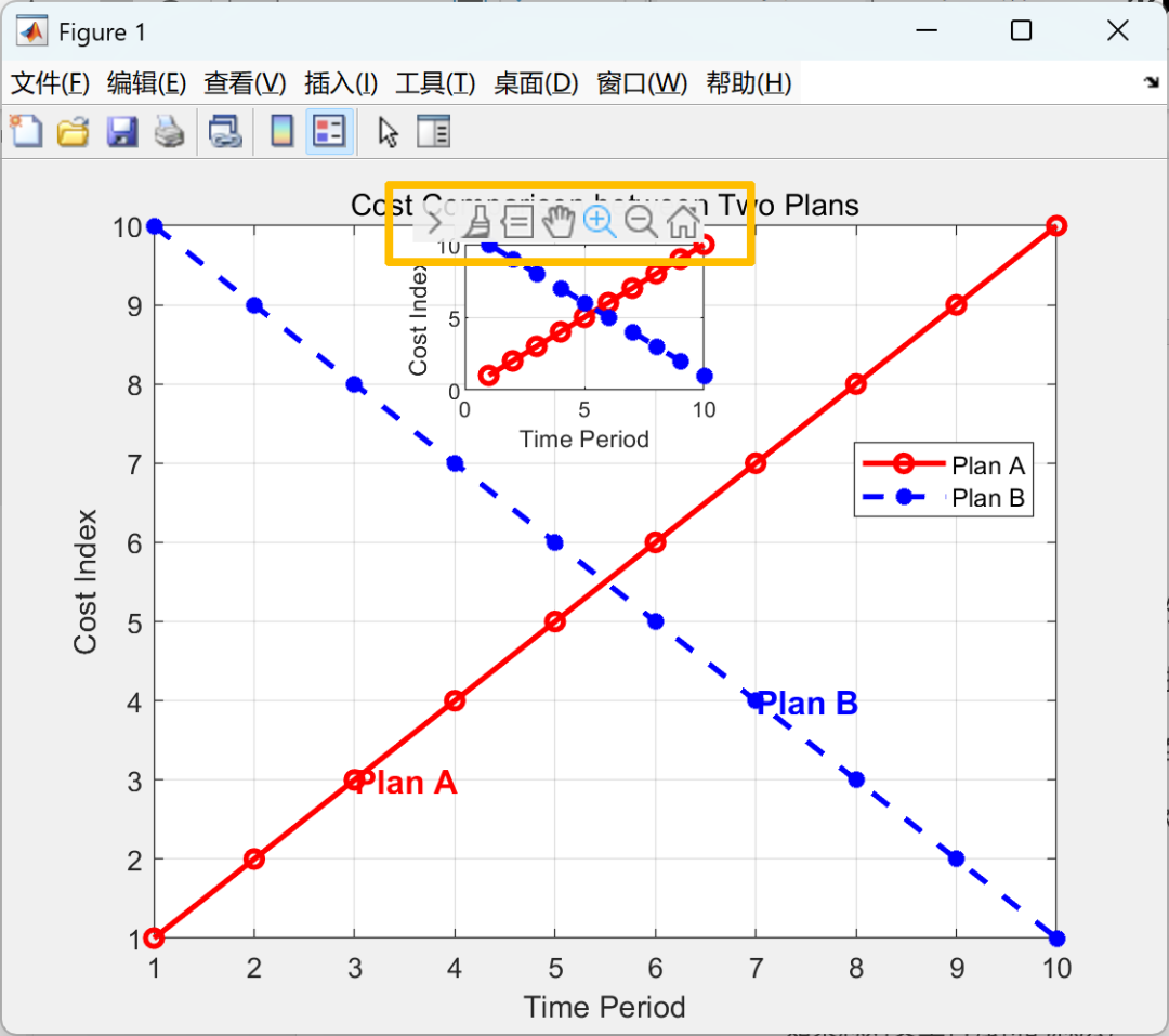
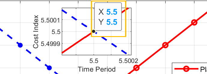
4. In the fourth step, we need to click on “Tools” > “Data Tips”. Then, place the mouse over the intersection point, right-click, and set the data display option to “Mouse Position” while adjusting it to an appropriate location. This allows us to mark the data at the intersection point.
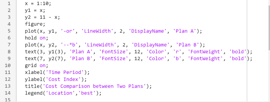
5. In the fifth step, we can utilize the gtext function or text function, as mentioned in the previous post, to add textual annotations.
6. Code and Final Image:
That’s all for today’s sharing.
If you have a unique idea about the article,
please leave us a message,
and let us meet tomorrow.
I wish you a nice day!
Translation: Wenxin Yiyan
References: Baidu, CSDN Community, ChatGPT, MATLAB Official Website
This article is organized and published by LearningYard Academy. If there is any infringement, please leave a message in the background!

Copywriter | Chen
Layout | Chen
Review | HZY