“ Using Shapely and Geopandas for PIP queries and intersection checks.”
Determining whether a point is inside a region, or whether a line intersects another line or a polygon, are fundamental topological operations. These operations have a wide range of applications, such as filtering data based on location. In spatial analysis, such spatial queries are often one of the typical initial steps in the workflow. Performing spatial joins between two spatial datasets is one of the most typical applications of checking whether a point is inside a polygon.
01
—
PIP (Point in Polygon) Query
From a computational perspective, determining whether a point is inside a polygon is a complex task. However, we can use built-in functions to perform the calculations and evaluate the topological relationships between geographic objects, such as the PIP (Point in Polygon) relationship.
There are two main methods to perform PIP queries in Shapely:
-
Using the within() function: This function checks whether a point is inside a polygon;
-
Using the contains() function: This function checks whether a polygon contains a point;
Additionally, the logic of PIP operations also applies to checking whether a LineString or a polygon is inside another polygon.
As an example, we first create a polygon using a set of coordinate tuples, and then create several point objects.
from shapely.geometry import Point, Polygon
p1 = Point(24.952242, 60.1696017)
p2 = Point(24.976567, 60.1612500)
coords = [(24.950899, 60.169158), (24.953492, 60.169158), (24.953510, 60.170104), (24.950958, 60.169990)]
poly = Polygon(coords)
We check whether the points are inside the polygon.
p1.within(poly)True
p2.within(poly)False
From this, we can see that the first point is inside the polygon, while the other point is not.
In fact, the first point is very close to the center of the polygon.
print(p1)POINT (24.952242 60.1696017)
print(poly.centroid)POINT (24.95224242849236 60.16960179038188)
We can also perform a PIP query in another way, which is to check whether a polygon contains a point.
poly.contains(p1)True
poly.contains(p2)False
The results of these two methods for checking spatial relationships are ultimately the same.
If we have multiple points and a polygon, and we want to determine which of these points are inside the polygon, we need to iterate through all the points and use the within() function to check each point against the specified polygon. If we have multiple polygons and a point, and we want to determine which polygon contains the point, we need to iterate through all the polygons and use the contains() function until we find a polygon that contains the specified point (assuming there are no overlapping polygons).
02
—
Intersection
Another typical topological operation is to determine whether one geometric object intersects (intersect) or touches (touch) another geometric object.
The difference between these two relationships is:
-
If two objects intersect (intersect), then the boundary and interior of one object must intersect with the boundary and interior of the other object in any way.
-
If one object touches (touch) another object, then they only need to have (at least) one common point on their boundaries, but their interiors must not intersect.
As an example, we first create two LineStrings.
from shapely.geometry import LineString, MultiLineString
line_a = LineString([(0, 0), (1, 1)])
line_b = LineString([(1, 1), (0, 2)])
Let’s check if they intersect.
line_a.intersects(line_b)TrueNow let’s check if they touch.
line_a.touches(line_b)TrueLet’s see if a LineString can touch itself.
line_a.touches(line_a)FalseNow let’s see if a LineString can intersect with itself.
line_a.intersects(line_a)True03
—
Using Geopandas for PIP Queries
We just used the Shapely package for topological calculations, now we will use Geopandas for related operations.
This time we will use aGeoPackage file as an example, which can still be downloaded from the following link:
https://pan.baidu.com/s/1bAnUo0S_ojxXdkyBqWAnLg?pwd=gxu2 Extraction code: gxu2
The example file contains observation records of protected species in a certain area, as well as a GeoJSON format polygon simulating the sub-basin of a river (which can also be downloaded from the above link). We will cross-check these two files to determine which observation records of protected species are located within the basin.
When reading layers from the GeoPackage file, we need to provide additional layer name information. This is because GeoPackage is essentially an embedded database format built on SQLite.
We first read the relevant data from this GeoPackage layer file.
import geopandas as gpd# Adjust the path according to the file storage location
species_fp = ".../species.gpkg"
species_data = gpd.read_file(species_fp, layer='category_3_species_porijogi', driver='GPKG')
We then read the GeoJSON file, which is the same as reading a Shapefile.
# Adjust the path according to the file storage location
polys_fp = ".../catchments.geojson"
polys = gpd.read_file(polys_fp, driver='GeoJSON')
Next, we filter for theIdaoja sub-basin, check its location, and plot the species observation points on the map layer.
import matplotlib.pyplot as plt
plt.style.use('ggplot')
plt.rcParams['figure.figsize'] = (15, 15)
subcatch = polys.loc[polys['NAME_1']=='Idaoja']
subcatch.reset_index(drop=True, inplace=True)
fig, ax = plt.subplots();
polys.plot(ax=ax, facecolor='gray')
subcatch.plot(ax=ax, facecolor='red')
species_data.plot(ax=ax, color='blue', markersize=5)
plt.tight_layout()
plt.show()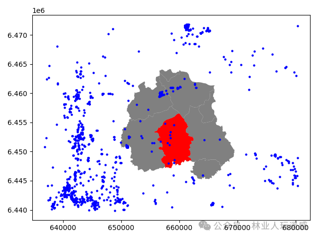
From this, we can see that some points are indeed located within the selected red polygon (sub-basin).
Next, we need to find out which points are located within this polygon, which requires performing a PIP query.
First, we enable shapely.speedups (the acceleration module of the Shapely library), which can speed up some spatial queries.
import shapely.speedups
shapely.speedups.enable()
We will check which points are within the subcatch polygon. Since we need to determine whether these points are within the geometry of the subcatch GeoDataFrame, we need to use loc[0, ‘geometry’] to extract the actual polygon geometry from the GeoDataFrame.
pip_mask = species_data.within(subcatch.loc[0, 'geometry'])
pip_mask0       False
1       False
2       False
3       False
4       False        ...  1032    False
1033    False
1034    False
1035    False
1036    False
Length: 1037, dtype: bool
Now we have a boolean array corresponding to each row of data: if a point is inside the polygon, the result is True; otherwise, it is False.
Next, we can use this mask array to filter out the points that are inside the polygon.
pip_data = species_data.loc[pip_mask]pip_data     OBJECTID        LIIK             NIMI   EXT_SYST_I    KKR_KOOD PRIV_TYYP
249    152958  taimed III    ohakasoomukas  -1902179792  KLO9331094    Avalik
674    145079  loomad III  valge-toonekurg  -1632330969  KLO9105497    Avalik
691    145191  loomad III  valge-toonekurg   1355787943  KLO9105625    Avalik
694    145194  loomad III  valge-toonekurg   1430734590  KLO9105624    Avalik
695    145196  loomad III  valge-toonekurg   1653031368  KLO9105598    Avalik
979    147275  loomad III  valge-toonekurg   -934352158  KLO9108256    Avalik
980    147279  loomad III  valge-toonekurg   -345614917  KLO9108257    Avalik
982    147282  loomad III  valge-toonekurg     13169300  KLO9108254    Avalik
985    147297  loomad III  valge-toonekurg   1849924613  KLO9108255    Avalik             STAATUS  IMPORT  LAADIMISKP                        geometry
249  kontrollitud       0  2018-10-29  POINT (657531.007 6454827.405)
674  kontrollitud       0  2018-10-29  POINT (657952.380 6451525.770)
691  kontrollitud       0  2018-10-29  POINT (659189.190 6448592.205)
694  kontrollitud       0  2018-10-29  POINT (658311.690 6451115.475)
695  kontrollitud       0  2018-10-29  POINT (658117.710 6447988.785)
979  kontrollitud       0  2018-10-29  POINT (659040.735 6454585.439)
980  kontrollitud       0  2018-10-29  POINT (658493.413 6453377.590)
982  kontrollitud       0  2018-10-29  POINT (658495.234 6452311.248)
985  kontrollitud       0  2018-10-29  POINT (658387.491 6452891.505)
Finally, we validate whether the PIP query executed successfully as expected by plotting the data.
subcatch = polys.loc[polys['NAME_1']=='Idaoja']
subcatch.reset_index(drop=True, inplace=True)
fig, ax = plt.subplots()
polys.plot(ax=ax, facecolor='gray')
subcatch.plot(ax=ax, facecolor='red')
pip_data.plot(ax=ax, color='gold', markersize=10)
plt.tight_layout()
plt.show()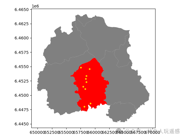
Now we see that the golden points are indeed all located within the red polygon, which is exactly the result we wanted.