This article uses the example of a cantilever beam subjected to a uniformly distributed load to demonstrate the implementation of MATLAB code from formula derivation to plotting!
1. Basic Idea:
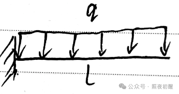
A cantilever beam subjected to a uniformly distributed load, which is fixed at one end and free at the other, has a length of L, an elastic modulus of E, and experiences a uniformly distributed load q, resulting in a deflection w(x).
The relationships between deflection w, angle θ, bending moment M, and shear force Q are as follows:
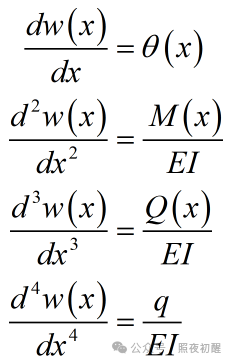
The specific approach is: based on the fourth-order derivative relationship between deflection w and load q, solve the differential equation, determine the unknowns using boundary conditions, and then calculate internal forces and plot the results based on other derivative relationships.
2. Code Implementation:
1. First, define the variables and use the dsolve function to solve the fourth-order ordinary differential equation.
syms w(x) q EI;dsolve(diff(w,x,4)==q/EI,x)The result is:
ans =(q*x^4)/(24*EI) + (C1*x^3)/6 + (C2*x^2)/2 + C3*x + C42. Then redefine new parameter variables and solve for the integration constants using boundary conditions.
syms x L q EI C1 C2 C3 C4;w=@(x)(q*x^4)/(24*EI) + (C1*x^3)/6 + (C2*x^2)/2 + C3*x + C4;w1(x)=diff(w(x),x,1);w2(x)=diff(w(x),x,2);w3(x)=diff(w(x),x,3);out=vpasolve(w(0)==0,w1(0)==0,w2(L)==0,w3(L)==0,C1,C2,C3,C4)The result is:
out = struct with fields: C1: -(L*q)/EI C2: (0.5*L^2*q)/EI C3: 0 C4: 03. Display all formulas based on the obtained results.
syms x L q EI;C1=-(L*q)/EI;C2=(0.5*L^2*q)/EI;C3=0;C4=0;w=@(x)(q*x^4)/(24*EI) + (C1*x^3)/6 + (C2*x^2)/2 + C3*x + C4;w1(x)=diff(w(x),x,1);w2(x)=diff(w(x),x,2);w3(x)=diff(w(x),x,3)The results are:
ans =(q*L^2*x^2)/(4*EI) - (q*L*x^3)/(6*EI) + (q*x^4)/(24*EI)
w1(x) =(q*L^2*x)/(2*EI) - (q*L*x^2)/(2*EI) + (q*x^3)/(6*EI)
w2(x) =(q*L^2)/(2*EI) - (q*L*x)/EI + (q*x^2)/(2*EI)
w3(x) =(q*x)/EI - (L*q)/EI
4. Substitute all formulas and plot the results.
syms x;q=1e6;L=10;E=5e9;h=4;EI=E*h^3/12;C1=-(L*q)/EI;C2=(0.5*L^2*q)/EI;C3=0;C4=0;w=@(x )(q*x^4)/(24*EI) + (C1*x^3)/6 + (C2*x^2)/2 + C3*x + C4;w1(x)=diff(w(x),x,1);w2(x)=diff(w(x),x,2);w3(x)=diff(w(x),x,3);rangeX=0:0.1:L;for i=1:length(rangeX) xi=rangeX(i); z(i) =double( w(xi)); z1(i)=double(w1(xi)); z2(i)=double(w2(xi)); z3(i)=double(w3(xi));endfigure(1)subplot(2,2,1)plot(rangeX,-z);title('Z')subplot(2,2,2)plot(rangeX,z1);title('theta')subplot(2,2,3)plot(rangeX,z2);title('M')subplot(2,2,4)plot(rangeX,z3);title('Q')The results are:
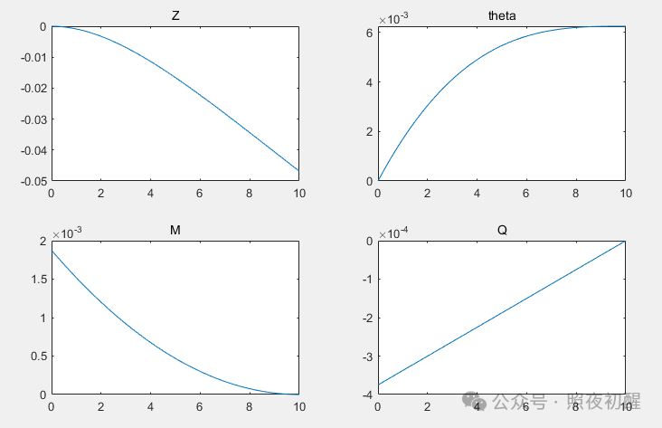
5. Thus, all objectives have been achieved. Here is all the code:
clear all;clc;close all;% syms w(x) q EI;% dsolve(diff(w,x,4)==q/EI,x)%q=1e6;L=10;E=5e9;h=4;EI=E*h^3/12;%============================================================% syms x L q EI C1 C2 C3 C4;% w=@(x)(q*x^4)/(24*EI) + (C1*x^3)/6 + (C2*x^2)/2 + C3*x + C4;% w1(x)=diff(w(x),x,1);% w2(x)=diff(w(x),x,2);% w3(x)=diff(w(x),x,3);% out=vpasolve(w(0)==0,w1(0)==0,w2(L)==0,w3(L)==0,C1,C2,C3,C4)%============================================================syms x;q=1e6;L=10;E=5e9;h=4;EI=E*h^3/12;C1=-(L*q)/EI;C2=(0.5*L^2*q)/EI;C3=0;C4=0;w=@(x )(q*x^4)/(24*EI) + (C1*x^3)/6 + (C2*x^2)/2 + C3*x + C4;w1(x)=diff(w(x),x,1);w2(x)=diff(w(x),x,2);w3(x)=diff(w(x),x,3);rangeX=0:0.1:L;for i=1:length(rangeX) xi=rangeX(i); z(i) =double( w(xi)); z1(i)=double(w1(xi)); z2(i)=double(w2(xi)); z3(i)=double(w3(xi));endfigure(1)subplot(2,2,1)plot(rangeX,-z);title('Z')subplot(2,2,2)plot(rangeX,z1);title('theta')subplot(2,2,3)plot(rangeX,z2);title('M')subplot(2,2,4)plot(rangeX,z3);title('Q')Thank you for reading!