
Let’s start with clock jitter measurement. The clock in discussion is a 133MHz clock with an amplitude of 150 mV and a duty cycle of 50%. To match the source impedance, the clock is connected to the oscilloscope using a 50-ohm coupling. Figure 1 shows the clock waveform displayed on the oscilloscope.
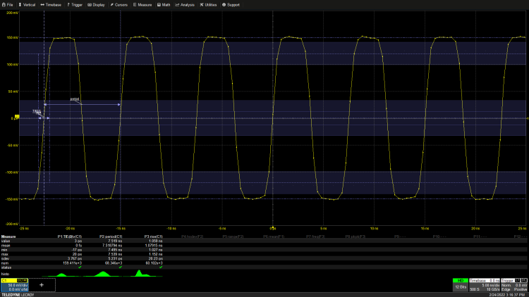 Figure 1: The 133 MHz clock showing measurement of time interval error, period, and rise time (including measurement statistics).
Measurement Parameters
The measurement parameters of the oscilloscope are used to quantify jitter. Two commonly used parameters are period and time interval error (TIE).
The period measures the time interval between adjacent edges with the same slope. The TIE parameter measures the time difference between the data edge and its ideal position. TIE can be considered as the instantaneous phase of the reported data stream. TIE measurements require knowledge of the clock frequency of the data stream, which can be explicitly input or determined by the oscilloscope during TIE establishment.
Measurement Statistics
In this case, the measurements of clock period, time interval error, and rise time are conducted over thousands of acquisition samples. The displayed measurement statistics include final measurement values, averages, minimums, maximums, standard deviation (sdev), and the number of statistical measurements. The oscilloscope records each measurement. Each acquisition display waveform contains five complete periods and seven rising edges, thus there are five period measurements and seven TIE and rise time measurements for each acquisition.
Standard deviation is a statistical figure that shows the distribution of measurement values around the mean. It is calculated by taking the measurement values (xi), subtracting the mean (µ), which essentially shows the instantaneous period jitter, and then squaring this difference. The average of the squared differences is calculated over the total number of measurements (N), and then the square root of this average is taken.
For periodic or TIE jitter associated with this clock signal, standard deviation is a good characterization. In fact, it is the root mean square (rms) value of periodic or TIE jitter. The difference between the maximum and minimum values is the peak jitter of the selected parameter.
Note the difference between the rms jitter of TIE and period. This difference is expected because TIE measures a single waveform edge, while period measures the difference between two edges. In such cases, the jitter on each edge is random and assumed to be independent, while the jitter in period measurement is the sum of the squares of the jitter on each edge. It is expected that the period jitter is approximately equal to the square root of 2 times the TIE jitter value.
Sampling Rate
Increasing rise time measurements ensures that the oscilloscope’s sampling rate is high enough to clearly define the edges of the clock signal. Each edge should have at least two samples. To have two samples within a 1ns rise time, the sampling rate should exceed 2GS/s.
The 50 nanosecond short record used in this measurement can display jitter variations at frequencies of 20 MHz or higher.
To match jitter with potential low-frequency sources, longer data records need to be acquired. This should be done while keeping the oscilloscope’s sampling rate fixed. This example uses a sampling rate of 10 gigasamples per second (GS/s), as the horizontal scale increases to 50 milliseconds per division, as shown in Figure 2.
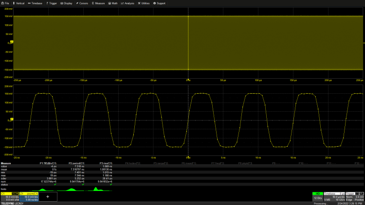
Figure 2: Increasing acquisition duration by extending the acquisition memory length to 5 million samples. The horizontal scale increases to 50 milliseconds per division.
This can measure jitter variations down to 2 kHz. The horizontal zoom trace Z1 is used to view parts of the waveform that were originally at 5ns per division and the actual acquisition. Even with long acquisitions, it is possible to measure TIE, period, and rise time of each cycle signal in the acquired clock signal. The standard deviation of the period is maintained at 5.2ps, while the standard deviation of TIE is maintained at 3.8ps.
For clock jitter, the choice between TIE or period measurement typically depends on the criteria of the user’s tests. Period-based jitter measurements are usually used to confirm clock signals. TIE measurements can be used for both clock and data signals.
Histogram
The icon below each measurement value represents the histogram of the measurement values. Clicking on this icon will display the histogram in the mathematical tracking, as shown in Figure 3.
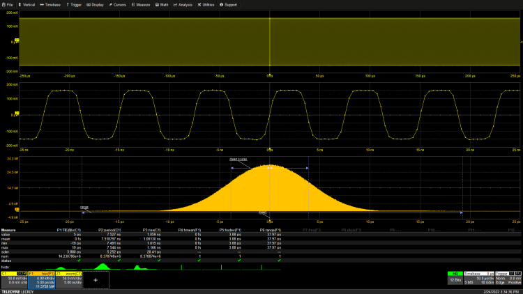
Figure 3: The histogram shows the distribution of the measured TIE values, with the shape of the distribution related to the source of jitter.
The histogram plots the number of measurement values within narrow ranges called bins. In this example, the histogram uses 2000 bins evenly spaced over a 50 ps window, so each bin has a width of about 25 fs. The shape of the histogram is related to the source of periodic jitter. The TIE values exhibit a bell shape characteristic of Gaussian or normal distribution. This type of distribution is associated with random processes such as noise. The histogram can be used to quantify parameters, in this case, the histogram adopts mean, standard deviation, and range. The blue line on the histogram marks the parameters, showing the measurement position of each parameter. As shown in Figure 3, for this Gaussian distribution, 68% of the measurements fall within ± 1 standard deviation of the mean. The lower the standard deviation, the closer it is to the mean of the measurement value distribution.
Tracking Function
The last tool in the basic jitter analysis toolbox is the tracking function. The tracking function plots the relationship of each measurement value over time. The trace is synchronized with the source waveform time, so each point on the trace corresponds to the measurement edge or period that produced that value occurring at the same time. Any periodic variation in the measured jitter will be displayed in the tracking function. In Figure 4, the TIE tracking function is added to the display screen.
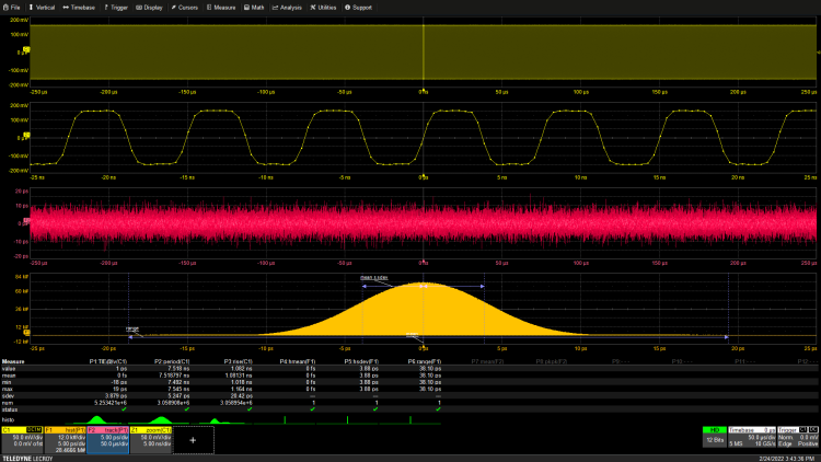
Figure 4: The tracking function shows the variation of TIE measurements over time, synchronized with the waveform acquired in channel C1.
The vertical scale of the TIE tracking function is in units of time, displaying the instantaneous deviation of each cycle of the acquired waveform from the ideal edge position. In this example, the trace is flat because the jitter is random noise with no apparent periodicity. If there is periodic jitter as shown in Figure 5, the trace will be more interesting.
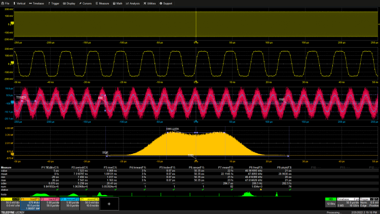
Figure 5: Measurement of a clock with both random and periodic TIE jitter components. The trace shows the time-varying periodic component.
By adding a 47kHz sine component to the clock jitter, the histogram will take on a bimodal shape. The histogram of the sine wave is saddle-shaped, convolving with the bell shape of the Gaussian distribution to form the observed bimodal shape. The separation of the peaks is proportional to the amplitude of the periodic jitter component. The tracking function reveals the shape of the sine jitter component added to the random component. The boxcar smoothing function applied to the trace on the trace function (the blue trace in mathematical trace F3) can attenuate the noise caused by random jitter components and display a smoothed version of the sine jitter component. Measurement parameters P7 and P8 read the frequency and peak amplitude of the periodic component, which are 47 MHz and 20 ps, respectively.
We performed some basic measurements of clock jitter using the jitter measurement tools in the oscilloscope. These measurements, after some modifications, can be used to measure the jitter of data signals, as shown in Figure 6.
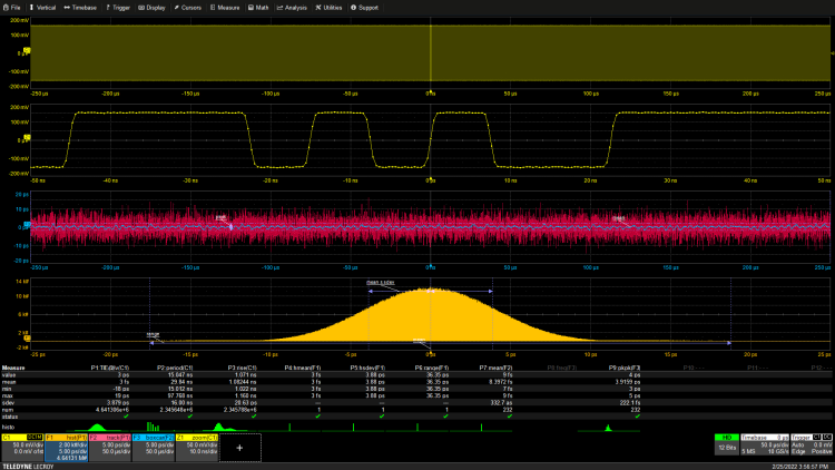
Figure 6: Jitter analysis of NRZ data signals using the time interval error parameter. The same tools used for analyzing clock jitter can also be used to measure jitter on data streams.
The NRZ data stream with a clock frequency of 133 MHz is the source of this analysis. The oscilloscope settings remain unchanged, with an acquisition window of 500ms and a sampling rate of 10 GS/s. The zoomed trace shows part of the PRBS 7 data. Unlike the clock waveform, the data waveform does not have a uniform period, so the period parameter is not applicable in jitter analysis. In the case of measuring clock jitter, data jitter will use the standard deviation of the TIE parameter as the rms value of the jitter measure. In this measurement, the standard deviation of TIE is 3.9 ps. The average value of TIE jitter is only 3 fs, indicating that the average jitter is close to zero.
As with clock jitter, the histogram and tracking tools provide additional insights. The histogram is centered around zero, consistent with the average value of the TIE parameter. The histogram range is 36 ps and is symmetrical around zero. The tracking function essentially shows a random variation around an average value that is roughly zero. The output of the overlaid boxcar filter shows a small peak-to-peak variation of 4 ps, even in the absence of periodic jitter. This is the result of data jitter related to the data stream. This is a form of deterministic jitter associated with the data pattern.
As with clock jitter, the histogram and tracking tools provide additional insights. As expected from the average value of the TIE parameter, the histogram is centered around zero. The histogram range is 36 ps and is essentially zero-symmetrical. The tracking function essentially shows a random variation around an average value that is about zero. Even without periodic jitter, the overlaid boxcar filter output shows small peak-to-peak variations of 4 ps. This is the result of jitter related to the data stream. This is a form of deterministic jitter associated with the data pattern.
If periodic jitter is added to the data stream, we will see results similar to those observed with clock jitter, as shown in Figure 7.
If periodic jitter is added to the data stream, we will also see results similar to those shown in Figure 7 for clock jitter.
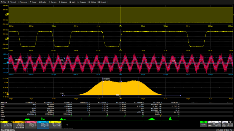
Figure 7: Jitter analysis of an NRZ data stream with random and periodic jitter components. Data-dependent jitter is also present.
The addition of periodic jitter elements causes the jitter histogram to become bimodal, as observed in the case of clock jitter. The tracking function shows the loss of the true sine waveform of the periodic jitter component. This is different from what happens when a periodic component is added to the clock waveform.
The distortion is due to the addition of data-dependent jitter, which is related to the data pattern. All these components are included in the standard deviation of the TIE measurement.
Basic jitter measurements start with the timing parameters TIE and period. The parameter statistics provide both rms and peak-to-peak jitter readings. The histogram of the parameters provides in-depth insights into the type of jitter and its distribution. Finally, the tracking function helps identify periodicities in jitter. Jitter measurements are taken from multiple measurement values reported in the statistical “num” field, which in most cases is less than 108.
Most oscilloscopes offer more advanced jitter analysis or serial data analysis software that can extrapolate measured jitter values and model jitter measurements of 1012 and higher. They also provide eye diagram displays with related eye diagram analysis. These features are typically very useful for consistency measurements of serial data.