Advanced Python Regression Prediction – Log Transformation of Target Variables

1. Why choose log transformation?

When we perform regression modeling,the target variable (the metric being predicted, such as house price SalePrice) does not conform to a normal distribution, we usually opt for log transformation, mainly for the following reasons:

1. Make the distribution closer to normal distribution

• Many real-world values (house prices, income, sales, population size, etc.) tend to have a right-skewed distribution (long tail):

• Most values are relatively small

• A few values are particularly large (“luxury houses”, “super-rich”, “hot-selling products”)

• A right-skewed distribution is detrimental to modeling because the model is easily affected by outliers.

• After log transformation, large values are “compressed”, and small values are “stretched”, making the distribution more symmetrical and closer to normal.

📌 Example: House prices range from 50,000 to 750,000. Without taking log, the model’s prediction errors are mainly concentrated on high-priced houses; after taking log, the price range is compressed to log(50k)≈10.8 to log(750k)≈13.5, reducing the impact of extreme values.

2. Stabilize variance (homoscedasticity)

• Linear regression and many machine learning models assume that the error term has homoscedasticity.

• If the target variable is right-skewed, typically the variance in the high-price range is greater than in the low-price range, leading to uneven prediction errors in the model.

• Log transformation can make the errors more uniform across different ranges, helping to improve the model’s fitting effect.

3. Improve model interpretability

• After taking the log, the meaning of the regression coefficients becomes “proportional/percentage change” rather than absolute change.

• This aligns better with conventions in economics, finance, and other fields.

• For example:<span><span>log(SalePrice)</span></span> a change of 0.1 corresponds to an increase in house price of about 10%, rather than a fixed increase of several thousand dollars.

4. Enhance model fitting and generalization ability

• Log transformation reduces the impact of extreme values → the model will not overly “chase” a few points like luxury houses → better generalization ability.

• In the Kaggle house price prediction competition, almost all excellent solutions will apply log transformation to the target SalePrice.

2. Specific exampleOK, let’s return to our project content: First, we will verify whether our sale price needs log transformation: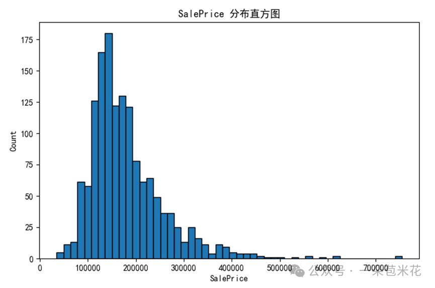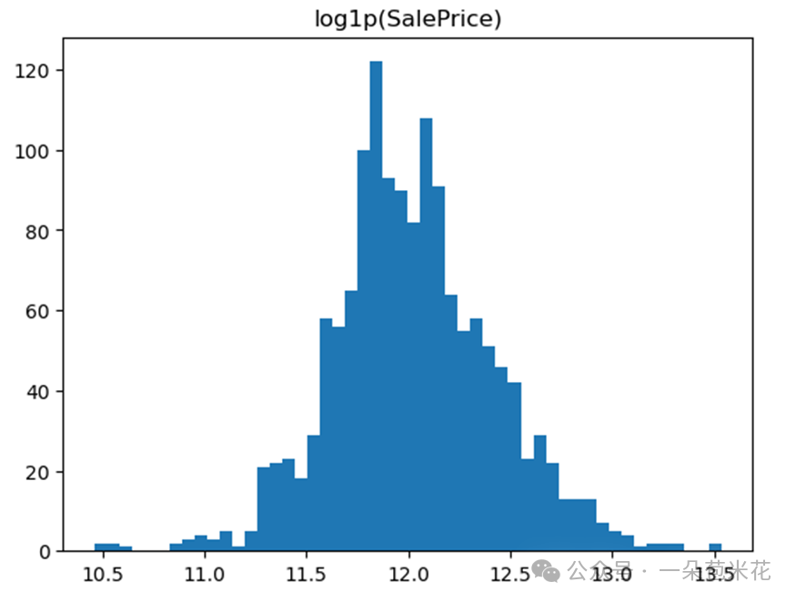Above are the histograms of the original data and the log-transformed “sale price”. The conclusions are as follows:

📊 1. Characteristics of the original distribution

Right-skewed distribution: From the first histogram, it can be seen that most house prices are concentrated between 100,000 ~ 200,000, but there are some high-priced houses (over 400,000, even 700,000+) that stretch the tail.

Long tail effect: A few high-priced houses have a significant impact on the mean, causing the average to be much higher than the median.Does not meet normality: The original SalePrice does not conform to a normal distribution, while many statistical modeling and machine learning algorithms (such as linear regression) often assume that residuals are close to normal distribution.

📊 2. log1p(SalePrice) Distribution characteristics

Close to normal distribution: After the log1p transformation, the data becomes symmetrical, resembling a bell curve, and is more consistent with normality.Reduces the impact of extreme values: Log transformation compresses the influence of high-priced houses, alleviating the long tail effect.Favorable for modeling:

• In regression models, the target value follows an approximately normal distribution, and the residuals will also be closer to normal, helping to improve model performance.
• In machine learning, the target value after log transformation often allows the model to be more stable and improves prediction accuracy.

📌Summary

• The original SalePrice: Right-skewed, long tail, not suitable for direct modeling.
• log1p(SalePrice): Approximately normal, more suitable as the target variable for regression models

3. Other methods to verify normal distributionps: This article discusses a small part of regression prediction modeling, so the example data connection can be found in another article: “Python Regression Prediction Modeling (reproducible, with all code, comments, and example dataset, House Prices + LightGBM + model interpretability)”. If you can’t find it, feel free to message me~The first method: D’Agostino and Pearson’s normality test (D’Agostino’s K² test or Omnibus K² test)

# Assuming you already have df, which contains SalePricesaleprice = df['SalePrice']
# Normality test (D'Agostino and Pearson's test)stat, p = stats.normaltest(saleprice)print('Statistic=%.3f, p=%.3f' % (stat, p))
if p > 0.05:    print("✅ SalePrice is approximately normally distributed")else:    print("❌ SalePrice does not conform to normal distribution")

The second method:Shapiro-Wilk normality test (Shapiro-Wilk test)

stat, p = stats.shapiro(saleprice)print('Statistic=%.3f, p=%.3f' % (stat, p))
if p > 0.05:    print("✅ SalePrice is approximately normally distributed")else:    print("❌ SalePrice does not conform to normal distribution")

The third method:Q-Q plot

import statsmodels.api as sm# Q-Q plotsm.qqplot(saleprice, line='s')plt.title("Q-Q Plot of SalePrice")plt.show()# If the points roughly fall on the straight line, it indicates closeness to normal distribution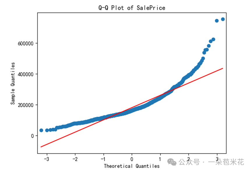

# Distribution after log transformationsaleprice_log = np.log1p(saleprice)
# Teststat, p = stats.normaltest(saleprice_log)print('Log1p(SalePrice) -> Statistic=%.3f, p=%.3f' % (stat, p))
# Q-Q plotsm.qqplot(saleprice_log, line='s')plt.title("Q-Q Plot of log1p(SalePrice)")plt.show()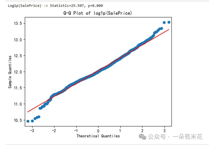

💬 Have you also completed this classic introductory problem? Feel free to leave a comment sharing your accuracy, code ideas, or experiences with pitfalls👇

❤️ If you find this useful, please support me:

– Give a “like” to encourage the author

– Share with friends who are learning machine learning

– Follow me to unlock more practical projects 🚀

📢 More exciting content

🔍 For systematic learning of data analysis and machine learning, project collaboration can be messaged to the public account

📬 Public account name: A Cornflower