Understanding TCP/IP Protocols in Depth

Click on the “Five-Minute Algorithm Learning” above to select the “Star” public account

Heavyweight content delivered first-hand Understanding TCP/IP Protocols in Depth

Understanding TCP/IP Protocols in Depth

From: Juejin, Author: Ruheng
Link: https://juejin.im/post/6844903490595061767

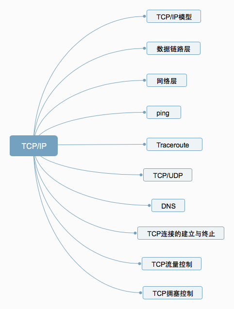
1. TCP/IP Model

The TCP/IP protocol model (Transmission Control Protocol/Internet Protocol) includes a series of network protocols that form the foundation of the internet and is the core protocol of the Internet.

The reference model based on TCP/IP divides the protocols into four layers: the Link Layer, Network Layer, Transport Layer, and Application Layer. The diagram below shows the correspondence between the TCP/IP model and the OSI model layers.

The TCP/IP protocol suite is layered from top to bottom, with each layer wrapping the one below it. The top layer is the Application Layer, which includes familiar protocols like HTTP and FTP. The second layer is the Transport Layer, where the well-known TCP and UDP protocols reside. The third layer is the Network Layer, where the IP protocol is responsible for adding IP addresses and other data to determine the transmission target. The fourth layer is the Data Link Layer, which adds an Ethernet protocol header to the data to be transmitted and performs CRC encoding to prepare for the final data transmission.

The above diagram clearly shows the function of each layer in the TCP/IP protocol, and the communication process of the TCP/IP protocol corresponds to the process of data being pushed onto and popped off the stack. During the push process, the sender at each layer continuously wraps headers and trailers, adding some transmission information to ensure delivery to the destination. During the pop process, the receiver at each layer continuously removes headers and trailers to obtain the final transmitted data.

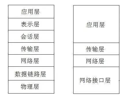
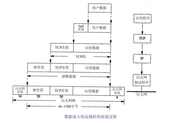
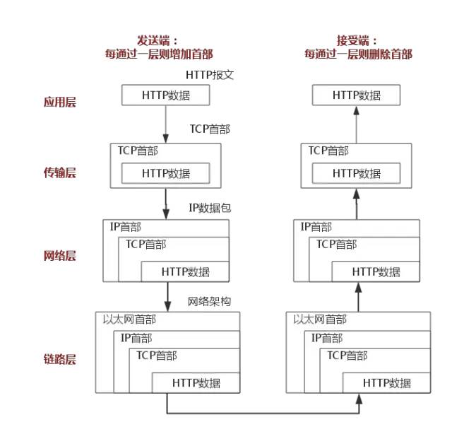
The above diagram uses the HTTP protocol as an example for further explanation.

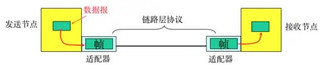
2. Data Link Layer

The Physical Layer is responsible for the interchange between the 0 and 1 bit streams and the physical device’s voltage levels and light flashes. The Data Link Layer is responsible for segmenting the 0 and 1 sequences into data frames for transmission from one node to a nearby node, which are uniquely identified by MAC addresses (MAC, physical address, each host has a MAC address).

Encapsulation into frames: Adding headers and trailers to the network layer datagram to encapsulate it into frames, with the frame header including the source MAC address and destination MAC address.
Transparent transmission: Zero bit padding, escape characters.
Reliable transmission: Rarely used on low-error-rate links, but wireless links (WLAN) ensure reliable transmission.
Error detection (CRC): The receiver checks for errors, and if an error is detected, the frame is discarded.

3. Network Layer

1. IP Protocol

The IP protocol is the core of the TCP/IP protocol, all TCP, UDP, ICMP, and IGMP data is transmitted in IP data format. It is important to note that IP is not a reliable protocol, meaning that the IP protocol does not provide a mechanism for handling undelivered data, which is considered the responsibility of upper-layer protocols: TCP or UDP.

1.1 IP Address

In the Data Link Layer, we generally identify different nodes by MAC addresses, while in the IP layer we also need a similar address identifier, which is the IP address.

A 32-bit IP address is divided into a network part and a host part, which reduces the number of entries in the routing table of routers. With a network address, we can limit terminals with the same network address to the same range, so the routing table only needs to maintain a single entry for that network address to reach the corresponding terminals.

Class A IP addresses: 0.0.0.0~127.0.0.0 Class B IP addresses: 128.0.0.1~191.255.0.0 Class C IP addresses: 192.168.0.0~239.255.255.0

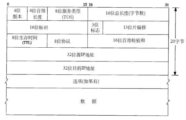
1.2 IP Protocol Header

This section only introduces the eight-bit TTL field. This field specifies how many routers the data packet can pass through before being discarded. Each time an IP data packet passes through a router, the TTL value decreases by 1, and when the TTL becomes zero, it is automatically discarded.

The maximum value of this field is 255, meaning that a protocol packet can pass through a router 255 times before being discarded. This number may vary depending on the system, generally being 32 or 64.

2. ARP and RARP Protocols

ARP is a protocol used to obtain MAC addresses based on IP addresses.

The ARP (Address Resolution Protocol) is a resolution protocol that allows a host to determine which interface corresponds to a given IP address. When a host wants to send an IP packet, it first checks its ARP cache (an IP-MAC address mapping table).

If the queried IP-MAC mapping does not exist, the host sends an ARP broadcast packet to the network containing the IP address to be queried. All hosts that receive this broadcast will check their IP addresses, and if one of the hosts finds it matches, it prepares an ARP packet containing its MAC address to send back to the broadcasting host.

Once the broadcasting host receives the ARP packet, it updates its ARP cache (which stores the IP-MAC mapping table). The broadcasting host will then use the new ARP cache data to prepare the data link layer packet for transmission.

The RARP protocol works oppositely and will not be elaborated upon here.

3. ICMP Protocol

The IP protocol is not a reliable protocol; it does not guarantee data delivery. Therefore, the responsibility of ensuring data delivery falls to other modules, with one important module being the ICMP (Internet Control Message Protocol). ICMP is not a high-level protocol but operates at the IP layer.

When errors occur in transmitting IP data packets, such as host unreachable or route unreachable, the ICMP protocol encapsulates the error information and sends it back to the host, providing the host with an opportunity to handle the error. This is why protocols built on top of the IP layer can achieve reliability.

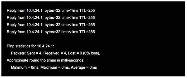
4. Ping

Ping can be considered the most famous application of ICMP and is part of the TCP/IP protocol. The “ping” command can check network connectivity and is very helpful for analyzing and diagnosing network issues.

For example, when we cannot access a certain website, we usually ping that website. Ping will echo some useful information. General information includes:

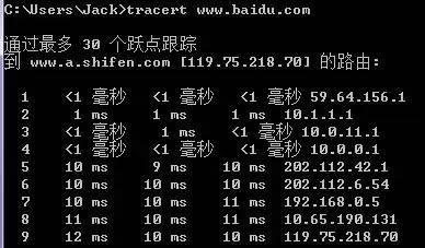
The word ping comes from sonar positioning, and this program indeed functions similarly, using ICMP packets to detect whether another host is reachable. The principle is to send a request with an ICMP type code of 0, and the responding host replies with an ICMP type code of 8.

5. Traceroute

Traceroute is an important tool for detecting the routing situation between a host and the destination host, and it is also one of the most convenient tools.

The principle of Traceroute is quite interesting. Upon receiving the destination host’s IP, it first sends a UDP packet with TTL=1 to the destination host. The first router that receives this packet automatically decreases the TTL by 1, and when the TTL becomes 0, the router discards the packet and generates an ICMP message indicating the host is unreachable. The host then receives this message and sends another UDP packet with TTL=2 to the destination host, prompting the second router to send an ICMP message back to the host. This process continues until the destination host is reached. In this way, Traceroute obtains the IPs of all the routers traversed.

6. TCP/UDP

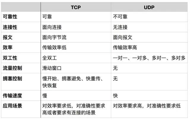
TCP and UDP are both transport layer protocols, but they have different characteristics and applications, analyzed in the table below.

Message-Oriented

In a message-oriented transmission mode, the application layer specifies the length of the message to UDP, and UDP sends it as is, one message at a time. Therefore, the application must choose an appropriate message size. If the message is too long, the IP layer needs to fragment it, reducing efficiency. If it is too short, it may be inefficient.

Byte Stream-Oriented

In a byte stream-oriented approach, although the application interacts with TCP one data block at a time (of varying sizes), TCP views the application as a continuous stream of unstructured bytes. TCP has a buffer, and when the data block sent by the application is too long, TCP can break it down into shorter segments before sending.

Congestion control and flow control are key aspects of TCP, which will be explained later.

Some applications of TCP and UDP protocols

When Should TCP Be Used?

When there are requirements for the quality of network communication, such as ensuring that all data is accurately transmitted to the other party, which is often used for reliable applications like file transfer protocols (HTTP, HTTPS, FTP) and email transmission protocols (POP, SMTP).

When Should UDP Be Used?

When there are no high requirements for network communication quality, and speed is prioritized, UDP can be used.

7. DNS

DNS (Domain Name System) is a distributed database on the Internet that maps domain names to IP addresses, allowing users to access the Internet more conveniently without having to remember machine-readable IP number strings. The process of obtaining the IP address corresponding to a hostname through the hostname is called domain name resolution (or hostname resolution). The DNS protocol operates over UDP, using port number 53.

8. Establishing and Terminating TCP Connections

1. Three-Way Handshake

TCP is connection-oriented, and before either party can send data, a connection must first be established between both parties. In the TCP/IP protocol, the TCP protocol provides reliable connection services, and the connection is initialized through a three-way handshake. The purpose of the three-way handshake is to synchronize the sequence numbers and acknowledgment numbers of both parties and exchange TCP window size information.

First Handshake: Establishing the connection. The client sends a connection request segment, setting SYN to 1 and Sequence Number to x; then, the client enters the SYN_SEND state, waiting for the server’s confirmation;

Second Handshake: The server receives the SYN segment. The server acknowledges the client’s SYN segment by setting Acknowledgment Number to x+1 (Sequence Number+1); at the same time, it sends its own SYN request, setting SYN to 1 and Sequence Number to y; the server puts all this information into a single segment (the SYN+ACK segment) and sends it to the client, entering the SYN_RECV state;

Third Handshake: The client receives the server’s SYN+ACK segment. It sets Acknowledgment Number to y+1 and sends an ACK segment to the server. After this segment is sent, both the client and server enter the ESTABLISHED state, completing the TCP three-way handshake.

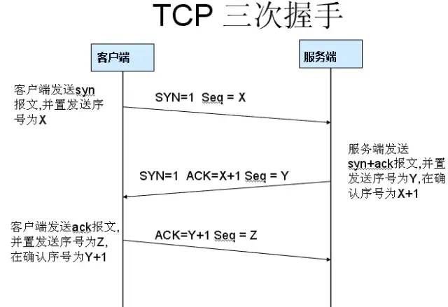
Why Three-Way Handshake?

To prevent a stale connection request segment from suddenly being sent to the server, causing errors.

Specific example: The generation of the “stale connection request segment” occurs in a situation where the first connection request segment sent by the client does not get lost but lingers at some network node for a long time, arriving at the server after the connection has already been released. This is an already invalid segment. However, when the server receives this stale connection request segment, it mistakenly believes it is a new connection request from the client.

Thus, it sends a confirmation segment back to the client, agreeing to establish the connection. If the “three-way handshake” is not used, as soon as the server sends a confirmation, the new connection would be established. Since the client has not sent a connection request, it will not respond to the server’s confirmation and will not send any data to the server. However, the server will think a new transport connection has been established and will wait for the client to send data, wasting many resources. The “three-way handshake” method prevents this phenomenon. For instance, in the previous case, the client would not respond to the server’s confirmation. The server, not receiving a confirmation, knows that the client did not request to establish a connection.

2. Four-Way Teardown

After the client and server have established a TCP connection through the three-way handshake, once the data transmission is complete, the TCP connection must be terminated. This is where the mysterious “four-way teardown” comes into play.

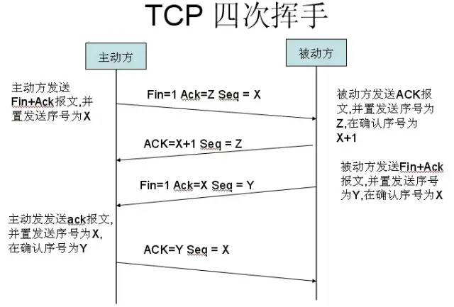
First Teardown: Host 1 (which can be either the client or server) sets the Sequence Number and sends a FIN segment to Host 2; at this point, Host 1 enters the FIN_WAIT_1 state; this indicates that Host 1 has no data to send to Host 2;

Second Teardown: Host 2 receives the FIN segment sent by Host 1 and responds with an ACK segment, setting Acknowledgment Number to the Sequence Number plus 1; Host 1 enters the FIN_WAIT_2 state; Host 2 informs Host 1 that it “agrees” to the close request; Third Teardown: Host 2 sends a FIN segment to Host 1, requesting to close the connection, and enters the LAST_ACK state;

Fourth Teardown: Host 1 receives the FIN segment sent by Host 2 and sends an ACK segment back to Host 2; then Host 1 enters the TIME_WAIT state; after Host 2 receives the ACK segment from Host 1, it closes the connection; at this point, Host 1 waits for 2MSL and, if no response is received, it confirms that the server has closed normally, allowing Host 1 to close the connection as well.

Why Four-Way Teardown?

The TCP protocol is a connection-oriented, reliable, byte stream-based transport layer communication protocol. TCP operates in full-duplex mode, which means that when Host 1 sends a FIN segment, it only indicates that Host 1 has no more data to send; Host 1 informs Host 2 that it has completed sending all its data; however, at this point, Host 1 can still receive data from Host 2. When Host 2 returns the ACK segment, it indicates that it has acknowledged that Host 1 has no data to send, but Host 2 can still send data to Host 1. When Host 2 also sends a FIN segment, it indicates that Host 2 also has no data to send, and it informs Host 1 that it has no data to send, after which both will happily terminate the TCP connection.

Why Wait for 2MSL?

MSL: Maximum Segment Lifetime, which is the longest time any segment can remain in the network before being discarded. There are two reasons for this:

To ensure that the TCP protocol’s full-duplex connection can be reliably closed
To ensure that any duplicate segments from this connection disappear from the network

The first point: If Host 1 directly goes to CLOSED, due to the unreliability of the IP protocol or other network reasons, Host 2 may not receive the final ACK from Host 1. Host 2, after a timeout, will continue to send FIN; at this point, since Host 1 has already CLOSED, it cannot find a corresponding connection for the retransmitted FIN. Therefore, Host 1 does not directly go to CLOSED but instead remains in TIME_WAIT, ensuring that the other party receives the ACK before finally closing the connection.

The second point: If Host 1 goes directly to CLOSED and then initiates a new connection to Host 2, we cannot guarantee that this new connection’s port number is different from the old one. That is, it is possible for the new connection and the old connection to have the same port number. Generally, this does not cause issues, but there can be special cases: if the new connection and the old closed connection have the same port number, and some delayed data from the previous connection arrives at Host 2 after the new connection is established, due to the same port numbers, TCP will consider that delayed data belongs to the new connection, causing confusion with the actual new connection’s data packets. Therefore, the TCP connection must wait in the TIME_WAIT state for 2MSL to ensure that all data from this connection disappears from the network.

9. TCP Flow Control

If the sender sends data too quickly, the receiver may not be able to keep up, leading to data loss. Flow control aims to ensure that the sender’s sending rate is not too fast, allowing the receiver to keep up with the reception.

Using the sliding window mechanism allows for easy flow control on a TCP connection.

Assuming A sends data to B. When the connection is established, B tells A: “My receive window is rwnd = 400” (where rwnd indicates the receiver window). Therefore, the sender’s sending window cannot exceed the value given by the receiver’s window. Note that the TCP window unit is bytes, not segments. Assume each segment is 100 bytes long, and the initial sequence number for the data segment is set to 1. Uppercase ACK indicates the acknowledgment bit in the header, while lowercase ack indicates the acknowledgment field value.

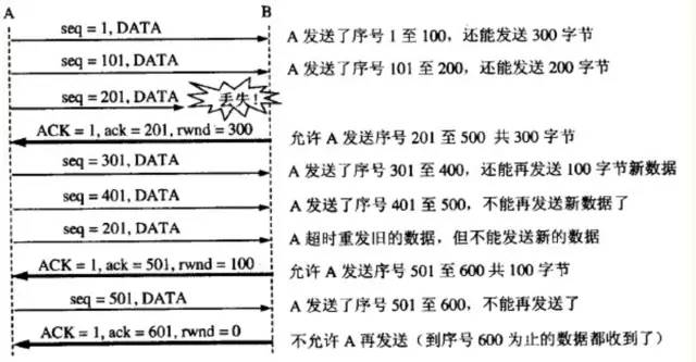
From the diagram, it can be seen that B performed flow control three times. The first time, it reduced the window to rwnd = 300, the second time to rwnd = 100, and finally to rwnd = 0, meaning that the sender is no longer allowed to send data. This state, where the sender is paused, will last until Host B sends a new window value.

TCP sets a persistent timer for each connection. Whenever one party in a TCP connection receives a zero window notification from the other party, it starts the persistent timer. If the timer expires, it sends a zero window probe segment (carrying 1 byte of data), prompting the other party to reset the persistent timer.

10. TCP Congestion Control

The sender maintains a congestion window (cwnd) state variable. The size of the congestion window depends on the level of network congestion and changes dynamically. The sender sets its sending window equal to the congestion window.

The principle for controlling the congestion window is: as long as there is no congestion in the network, the congestion window will increase to send more packets. However, if congestion occurs, the congestion window will decrease to reduce the number of packets injected into the network.

The slow start algorithm:

When a host starts sending data, if a large amount of data is injected into the network immediately, it may cause network congestion, as the current load of the network is unknown. Therefore, a better approach is to probe first, gradually increasing the sending window from small to large, that is, increasing the congestion window value gradually.

Typically, when starting to send segments, the congestion window cwnd is initially set to the size of one Maximum Segment Size (MSS). For every new acknowledgment received for a segment, the congestion window increases by at most one MSS. This gradual increase of the sender’s congestion window cwnd allows for a more reasonable rate of packet injection into the network.

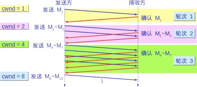
Each transmission round doubles the congestion window cwnd. The time for a transmission round is essentially the round-trip time RTT. However, “transmission round” emphasizes that all segments allowed to be sent by the congestion window cwnd are sent continuously until the acknowledgment for the last byte sent is received.

Also, the “slow” in slow start does not refer to the slow growth rate of cwnd, but rather that when TCP starts sending segments, it initially sets cwnd=1, allowing the sender to send only one segment (to probe the network’s congestion situation), and then gradually increases cwnd.

To prevent the congestion window cwnd from growing too large and causing network congestion, a slow start threshold (ssthresh) state variable must also be set. The usage of the slow start threshold ssthresh is as follows:

When cwnd < ssthresh, use the slow start algorithm described above.
When cwnd > ssthresh, stop using the slow start algorithm and switch to the congestion avoidance algorithm.
When cwnd = ssthresh, either the slow start algorithm or the congestion control avoidance algorithm can be used.

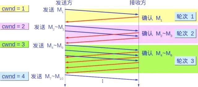
Congestion Avoidance

The congestion window cwnd is increased slowly, that is, for every round-trip time RTT, the sender’s congestion window cwnd increases by 1, rather than doubling. This causes the congestion window cwnd to grow slowly in a linear fashion, much slower than the growth rate of the congestion window in the slow start algorithm.

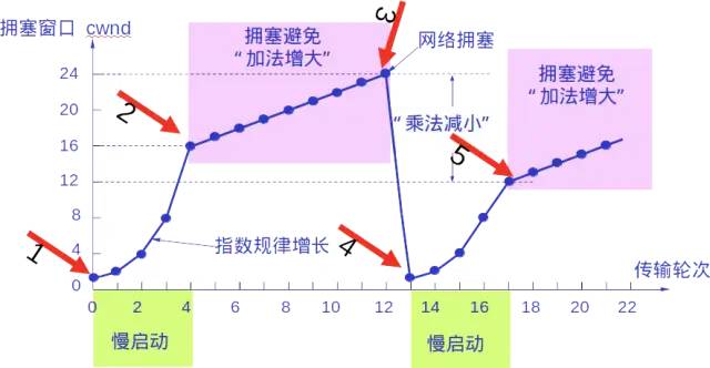
Whether in the slow start phase or the congestion avoidance phase, as soon as the sender detects network congestion (indicated by not receiving acknowledgments), it should set the slow start threshold ssthresh to half the value of the sender window at the time of congestion (but not less than 2). Then, it should reset the congestion window cwnd to 1 and execute the slow start algorithm.

The purpose of this approach is to quickly reduce the number of packets sent into the network, allowing the congested routers enough time to process the queued packets.

The following diagram illustrates the process of congestion control with specific values. The size of the sending window is equal to that of the congestion window.

2. Fast Retransmit and Fast Recovery

Fast Retransmit

The fast retransmit algorithm requires the receiver to immediately send a duplicate acknowledgment (to inform the sender that a segment has not been received) whenever it receives a segment out of order, rather than waiting until it sends data to include the acknowledgment.

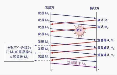
After the receiver receives M1 and M2, it sends acknowledgments for both. Now assume the receiver did not receive M3 but subsequently received M4.

Clearly, the receiver cannot acknowledge M4 because it is an out-of-order segment. According to the reliable transmission principle, the receiver can either do nothing or send a duplicate acknowledgment for M2 at an appropriate time.

However, according to the fast retransmit algorithm, the receiver should promptly send a duplicate acknowledgment for M2, allowing the sender to know that segment M3 has not reached the receiver. The sender then transmits M5 and M6. The receiver receives these two segments and must also send another duplicate acknowledgment for M2. In this way, the sender receives four acknowledgments for M2 from the receiver, the last three of which are duplicates.

The fast retransmit algorithm also stipulates that the sender should immediately retransmit the unacknowledged segment M3 as soon as it receives three duplicate acknowledgments, without waiting for the retransmission timer for M3 to expire.

By retransmitting unacknowledged segments early, the overall network throughput can increase by about 20%.

Fast Recovery

Fast recovery algorithm is used in conjunction with fast retransmit, and it has the following two key points:

When the sender receives three consecutive duplicate acknowledgments, it executes the “multiplicative decrease” algorithm, halving the slow start threshold ssthresh.
Unlike slow start, the sender does not set cwnd to 1 but instead sets it to the value of ssthresh halved, and then begins to execute the congestion avoidance algorithm (“additive increase”), allowing the congestion window to increase slowly in a linear fashion.