Please respect the original work.Please indicate the link to this article when reproducing.Author: slandarer
Hello, it’s been a long time! In this issue, we will create a radar chart similar to the one from Nature. The original image is shown below:
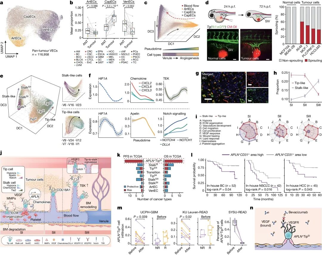
This image is from:
- Pan, X., Li, X., Dong, L. et al. Tumour vasculature at single-cell resolution. Nature 632, 429–436 (2024). https://doi.org/10.1038/s41586-024-07698-1
The reproduction effect for this issue is as follows:
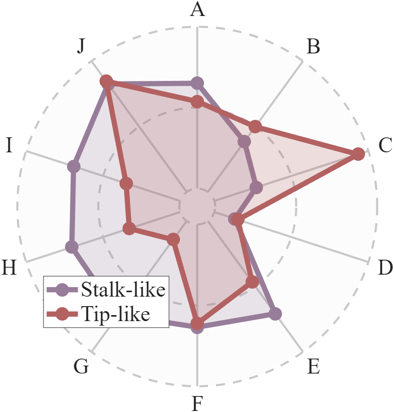
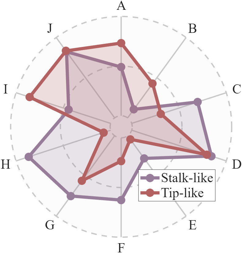
This reproduction is essentially a functional development of the radar chart tool I wrote a long time ago, which can be found on File Exchange:
- https://www.mathworks.com/matlabcentral/fileexchange/126450-radar-chart
Of course, I will also upload the tool and complete code to the Gitee platform and share the link at the end of this article. Let’s start with the main content, first, here is the basic usage of the tool:
X=randi([2,8],[4,7])+rand([4,7]); % Randomly generate data
RC=radarChart(X); % Generate radar chart object
RC.PropName={'Modeling','Experiment','Programming','Summary','Writing','Innovation','Leisure'};
RC.ClassName={'Peer A','Peer B','Peer C','Peer D'};
RC=RC.draw(); % Draw the chart
RC=RC.legend(); % Add legend
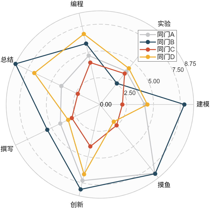
As you can see, the usage is very simple. Now let’s start reproducing the Nature plot:
Main Content
0. Data Preparation and Object Creation
figure('Position',[600,200,600,600]);

Data1 = rand([2,10]);
RC = radarChart(Data1);
1. Basic Settings and Plotting
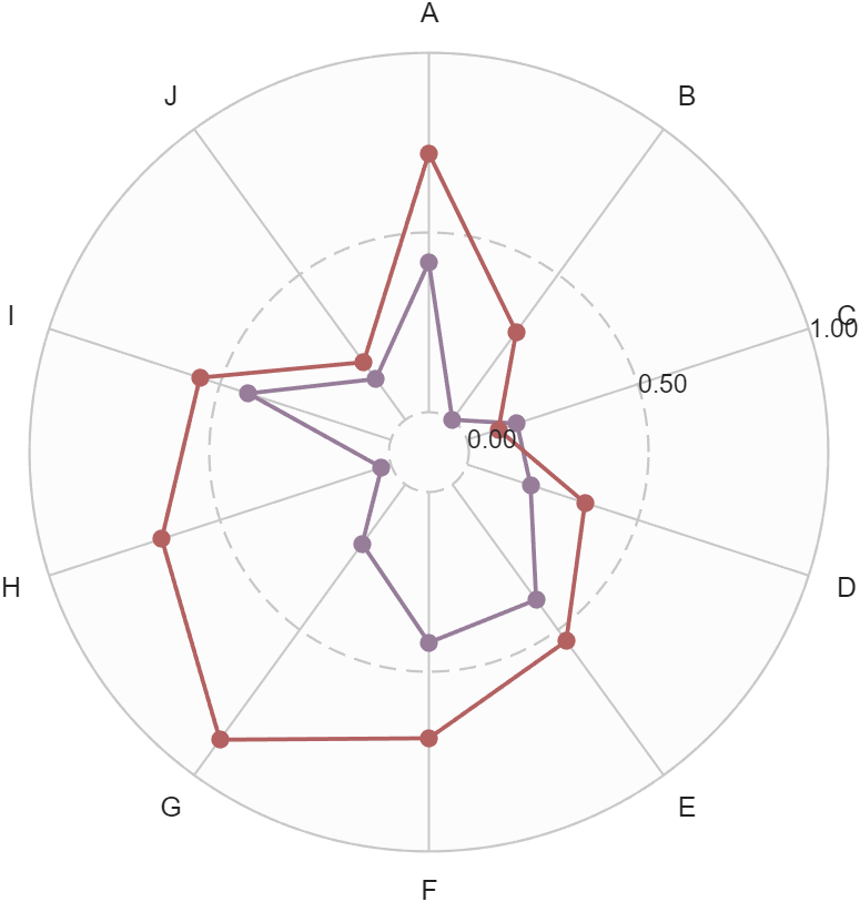
This includes information such as scale range, background coverage, initial angle, and whether labels are arranged clockwise or counterclockwise, as well as variable names and color schemes.
RC.RLim = [0,1];         % Set data range to 0,1
RC.RTick = [0,.5,1];     % Set radius ticks at 0, 0.5, and 1
RC.RRange = [.1,1];      % Set the range for the background (0.1 to 1)
RC.Rotation = pi/2;      % Set the initial angle
RC.ThetaDir = 'reverse'; % Set the direction of the label arrangement (counterclockwise or clockwise)

% Set variable names
RC.ClassName = {'Stalk-like','Tip-like'};
RC.PropName = num2cell('A':'J');
% RC.PropName = {'A','B','C','D','E','F','G','H','I','J'}
RC.CList = [151,125,154; 179,97,97]./255;

RC = RC.draw();
2. Modifying Background and Scale Lines and Labels
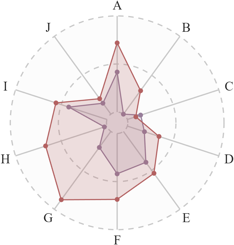
% Set background line thickness and other properties
RC.setPropLabel('FontSize',21,'FontName','Times New Roman');
RC.setRTick('LineWidth',2);
RC.setRLabel('Color','none');
RC.setBkg('EdgeColor','none');
RC.setThetaTick('LineWidth',2);
RC.setType('Both')
3. Modifying the Chart and Adding a Legend
RC.setPatchN(1, 'LineWidth',5, 'MarkerSize',8);
RC.setPatchN(2, 'LineWidth',5, 'MarkerSize',8);

RC = RC.legend();
RC.setLegend('FontSize',21, 'FontName','Times New Roman');
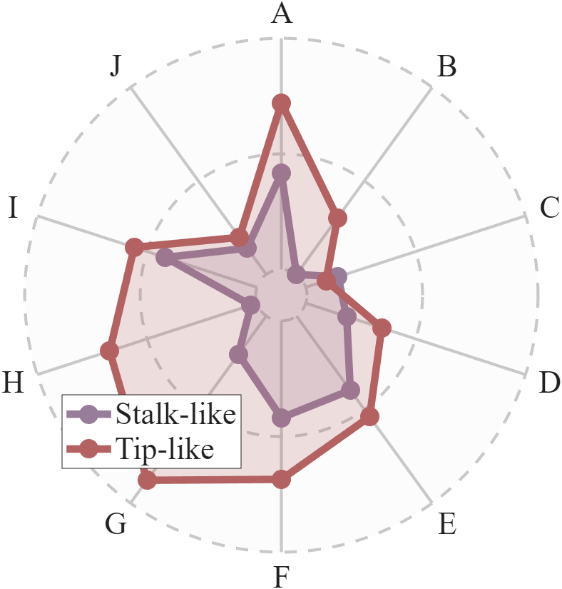
End
This plotting is still very simple. The complete code for this article has been uploaded to the Gitee repository:
- https://gitee.com/slandarer/PLTreprint