In a Battery Management System (BMS), the State of Charge (SOC) is a key indicator that describes the remaining battery capacity. Accurately predicting SOC is crucial for battery efficiency and safety. This article will introduce how to implement precise SOC prediction using the Support Vector Regression (SVR) model, showcasing the entire process from data processing to model evaluation with complete code.
What is SVR?
Support Vector Regression (SVR) is a regression algorithm based on Support Vector Machines, particularly suitable for handling data with nonlinear relationships. Compared to traditional regression methods, SVR has the following advantages:
- Effectively handles high-dimensional feature spaces
- Easily addresses nonlinear problems through kernel functions
- Insensitivity to noisy data
- Performs excellently on small sample datasets
These characteristics make SVR an ideal choice for predicting battery SOC, as there exists a complex nonlinear relationship between battery voltage, current, and SOC.
Complete Implementation Process
The SOC prediction scheme mainly includes the following steps:
- Data loading and preprocessing
- Dataset splitting (training set and test set)
- SVR model construction and hyperparameter optimization
- Model evaluation and performance metric calculation
- Prediction result visualization
First, necessary Python libraries need to be imported, and the battery dataset loaded:
import pandas as pd
import numpy as np
import matplotlib.pyplot as plt
from sklearn.svm import SVR
from sklearn.model_selection import GridSearchCV
from sklearn.preprocessing import StandardScaler
from sklearn.metrics import mean_squared_error, mean_absolute_error, r2_score
import joblib
# Load dataset
data = pd.read_csv('battery_data.csv')
2. Data Preprocessing and Splitting
Feature normalization is a key step before training the SVR model, which can effectively improve model performance:
# Extract features and target variable
X = data[[...]].values
y = data['SOC_scaled'].values
# Feature normalization
scaler = StandardScaler()
X_normalized = scaler.fit_transform(X)
# Split training and test sets (80:20 ratio)
n = X.shape[0]
train_ratio = 0.8
train_size = round(train_ratio * n)
X_train = X_normalized[:train_size, :]
y_train = y[:train_size]
X_test = X_normalized[train_size:, :]
y_test = y[train_size:]
Why Normalize? SVR is sensitive to the scale of features; normalization can convert features of different magnitudes to the same scale, avoiding excessive influence of certain features on the model.
3. SVR Model Construction and Hyperparameter Optimization
The performance of the SVR model largely depends on hyperparameter selection, optimized using Grid Search (GridSearchCV):
# Define hyperparameter search space
param_grid = {    'C': [0.1, 1, 10, 100],  # Regularization parameter
    'epsilon': [0.01, 0.1, 0.2],  # Insensitive loss function parameter}
best_models = {}
predictions = {}
metrics = {}
# Define scoring methods
scoring_methods = {    'neg_mse': 'neg_mean_squared_error'}
# Grid search to optimize model
for name, scoring in scoring_methods.items():    print(f"\nUsing scoring method: {name}")
    # Initialize SVR model (using RBF kernel to handle nonlinear relationships)
    svr = SVR(kernel='rbf')
    # Grid search
    grid_search = GridSearchCV(        estimator=svr,        param_grid=param_grid,        cv=5,  # 5-fold cross-validation        scoring=scoring,        verbose=1,        n_jobs=-1  # Use all available CPUs    )
    # Train model    grid_search.fit(X_train, y_train)
    # Get best model    best_model = grid_search.best_estimator_    best_models[name] = best_model    print(f"{name} best hyperparameters: {grid_search.best_params_}")
Key Hyperparameter Explanation:
- C: Regularization parameter that controls the balance between model complexity and generalization ability
- epsilon: Defines the insensitive zone, controlling the model’s tolerance for errors
- kernel=’rbf’: Uses radial basis function to handle nonlinear relationships between features
4. Model Evaluation and Performance Metrics
After training, the model’s performance needs to be evaluated on the test set:
# Make predictions on the test set
y_pred = best_model.predict(X_test)
predictions[name] = y_pred
# Calculate evaluation metrics
mse = mean_squared_error(y_test, y_pred)
rmse = np.sqrt(mse)  # Root Mean Square Error
mae = mean_absolute_error(y_test, y_pred)  # Mean Absolute Error
r2 = r2_score(y_test, y_pred)  # R-squared
# Save evaluation results
metrics[name] = {    'rmse': rmse,    'mae': mae,    'r2': r2}
# Output evaluation results
print(f'{name} Root Mean Square Error (RMSE): {rmse:.4f}')
print(f'{name} Mean Absolute Error (MAE): {mae:.4f}')
print(f'{name} R² Score: {r2:.4f}')
Interpretation of Evaluation Metrics:
- RMSE (Root Mean Square Error): Reflects the average deviation between predicted and actual values; the smaller the value, the better
- MAE (Mean Absolute Error): Reflects the average absolute difference between predicted and actual values; the smaller the value, the better
- R² (R-squared): Measures the model’s ability to explain data variability; the closer to 1, the better the model performance
5. Prediction Result Visualization
To visually demonstrate the model’s effectiveness, a comparison between actual SOC values and predicted values will be made:
plt.figure(figsize=(12, 7))
# Plot actual and predicted values
plt.plot(y_test, 'b-', linewidth=1.5, label='Actual SOC')
plt.plot(predictions['neg_mse'], 'r--', linewidth=1.5, label='Predicted SOC')
# Chart settings
plt.xlabel('Sample Index', fontsize=12)
plt.ylabel('SOC (%)', fontsize=12)
plt.title('SVR Model SOC Prediction Results', fontsize=14)
plt.legend(fontsize=10)
plt.grid(True, linestyle='--', alpha=0.7)
plt.tight_layout()
# Save and display chart
plt.savefig('soc_prediction_comparison.png', dpi=300)
plt.show()
Visualization Effect:
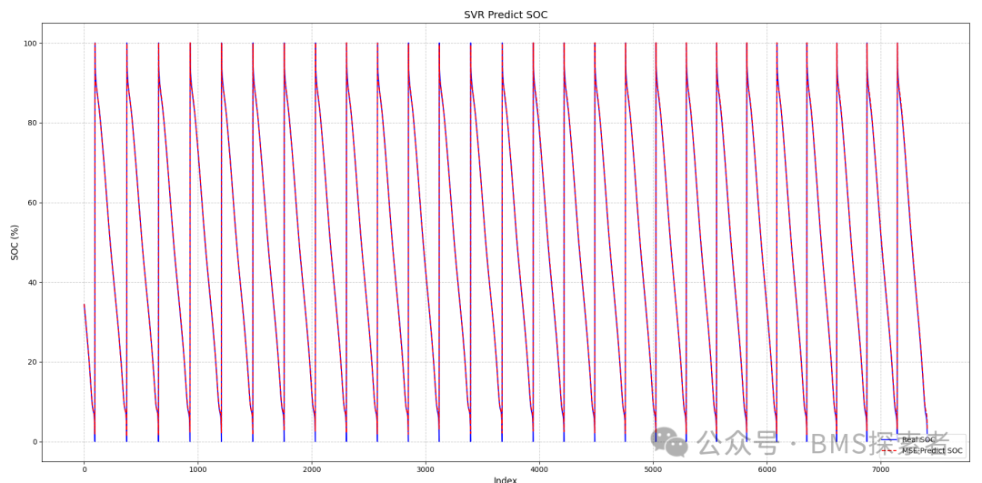
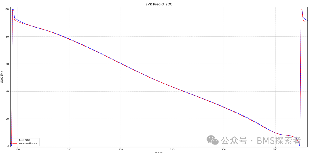
- The blue solid line represents the actual SOC value of the battery
- The red dashed line represents the predicted SOC value by the model
- The closer the two lines are, the better the prediction performance