Original link: http://tecdat.cn/?p=24092

In quantitative finance, I have learned various time series analysis techniques and how to use them (click the “Read the original” link at the end for the complete code data).

Related Videos

By developing our time series analysis (TSA) method combinations, we can better understand what has happened and make better, more favorable predictions about the future. Example applications include forecasting future asset returns, future correlations/covariances, and future volatilities.

Before we begin, let’s import our Python libraries.

import pandas as pd
import numpy as np

Let’s use the pandas package to fetch some sample data via API.

# Raw adjusted closing prices
daa = pdDatrme({sx(sm)for sm i syos})
# Log returns
ls = log(dta/dat.sit(1)).dropa()

Basic Knowledge

What is a Time Series?

A time series is a series of data points indexed in time order. — Wikipedia

Stationarity

Why do we care about stationarity?

• Stationary time series (TS) are easy to predict because we can assume that future statistical properties are the same or proportional to current statistical properties.

• Most models we use in TSA assume covariance stationarity. This means that the descriptive statistics (e.g., mean, variance, and correlation) predicted by these models are only reliable when the TS is stationary; otherwise, they are invalid.

“For example, if a sequence continuously increases over time, the sample mean and variance will grow with the sample size, and they will always underestimate the mean and variance of future periods. If a sequence’s mean and variance are not clearly defined, then its correlation with other variables is also not.”

That said, most TS we encounter in finance are not stationary. Therefore, a large part of TSA involves identifying whether the sequence we want to predict is stationary, and if not, we must find ways to transform it into a stationary one (which will be detailed later).

Autocorrelation

Essentially, when we model a time series, we decompose the sequence into three parts: trend, seasonality/cyclicality, and randomness. The random component is called the residual or error. It is simply the difference between our predicted values and observed values. Serial correlation refers to the correlation of the residuals (errors) of our TS model with each other.

Why do we care about serial correlation?

We care about serial correlation because it is crucial for the validity of our model predictions and is intrinsically linked to stationarity. Recall that by definition, the residuals (errors) of a stationary TS are continuously uncorrelated! If we do not account for this in our model, the standard errors of our coefficients will be underestimated, exaggerating our T-statistics. The result is too many Type I errors, where we reject the null hypothesis even when it is true! In layman’s terms, ignoring autocorrelation means our model predictions will be nonsense, and we may draw incorrect conclusions about the effects of independent variables in the model.

White Noise and Random Walks

White noise is the first time series model (TSM) we need to understand. By definition, a time series that is a white noise process has continuously uncorrelated errors, with an expected mean of zero. Another way to describe continuously uncorrelated errors is that they are independent and identically distributed (i.i.d.). This is important because if our TSM is appropriate and successfully captures the underlying process, the residuals of our model will be i.i.d., similar to a white noise process. Therefore, part of TSA is actually trying to fit a model to the time series such that the residual sequence is indistinguishable from white noise.

Let’s simulate a white noise process and take a look at it. Below, I introduce a convenient function for plotting time series and visually analyzing serial correlation.

We can easily model a white noise process and output a TS plot for inspection.

np.random.seed(1)

# Plotting discrete white noise curve
ads = radooral(size=1000)
plot(ads, lags=30)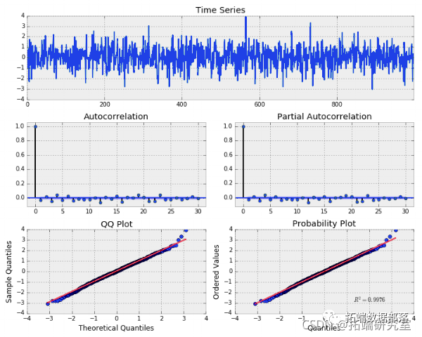

Gaussian White Noise

We can see that the process appears to be random and centered around zero. The autocorrelation (ACF) and partial autocorrelation (PACF) plots also indicate no significant serial correlation. Remember, we should see about 5% significance in the autocorrelation plot, which is due to pure chance from sampling from a normal distribution. Below, we can see QQ and probability plots that compare our data distribution with another theoretical distribution. In this case, the theoretical distribution is the standard normal distribution. Clearly, our data is randomly distributed and should follow Gaussian (normal) white noise.

p("nmean: {:.3f}\{:.3f}\stde: {:.3f}".format(ademean(), nerva(), der.td()))

The significance of random walks is that they are non-stationary because the covariance between observations is time-dependent. If the TS we are modeling is a random walk, it is unpredictable.

Let’s simulate a random walk using the “random” function sampled from the standard normal distribution.

# Random walk without drift
np.rao.sed(1)
n = 1000

x = w = np.aonral(size=n)
for t in rnge(_sples):
    x[t] = x[t-1] + w[t]
splt(x, las=30)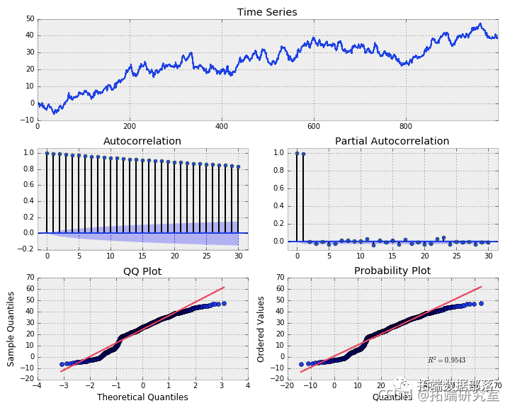

Random Walk Without Drift

Clearly, our TS is not stationary. Let’s see how well the random walk model fits our simulated data. Recall that a random walk is xt = xt-1 + wt. Using algebra, we can say xt – xt-1 = wt. Therefore, the first difference of our random walk series should equal a white noise process, and we can use the np.diff() function on our TS to see if this holds.

# First difference of simulated random walk
plt(p.dffx), las=30)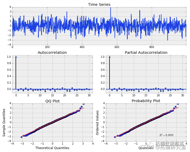

First Difference of Random Walk

Our definition holds because this looks exactly like a white noise process. What if we take the first difference of the SPY prices for a random walk?

Click the title to check past content

R Language ARIMA-GARCH Volatility Model Forecasting Stock Market Daily Returns Time Series for Apple Inc.

Swipe left to see more

01

02

03

04

# First difference of SPY prices
plt(diff(dt.PY), lag=30)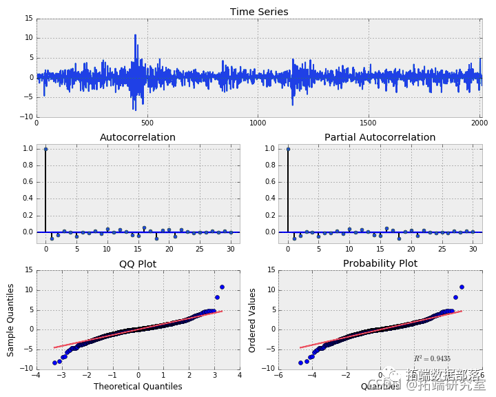

Fitting Random Walk Model to ETF Prices

It is very similar to white noise. However, note the shape of the QQ and probability plots. This indicates that the process is close to a normal distribution but has “heavy tails.” The ACF and PACF also seem to show some significant serial correlation around lags 1, 5, 16, 18, and 21. This suggests that there should be a better model to describe the actual price change process.

Linear Models

Linear models, also known as trend models, represent a TS that can be plotted with a straight line. The basic equation is as follows:

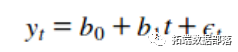
In this model, the value of the dependent variable is determined by the β coefficients and a single independent variable—time. An example is that a company’s sales increase by the same amount in each time period. Let’s look at a specially crafted example below. In this simulation, we assume that the steadfast ABC company has sales of -50.00 (β0 or intercept term) and +25.00 (β1) in each time step.

# Simulating linear trend
# Example: Company ABC's sales default to -50, increasing by +25 in each time step
w = n.anom.ann(100)
y = nppt_lke(w)

b0 = -50.
b1 = 25.
for t in rge(lnw)):
    y[t] = b0 + b1*t + w[t]
    
 plt(y, lags=ls)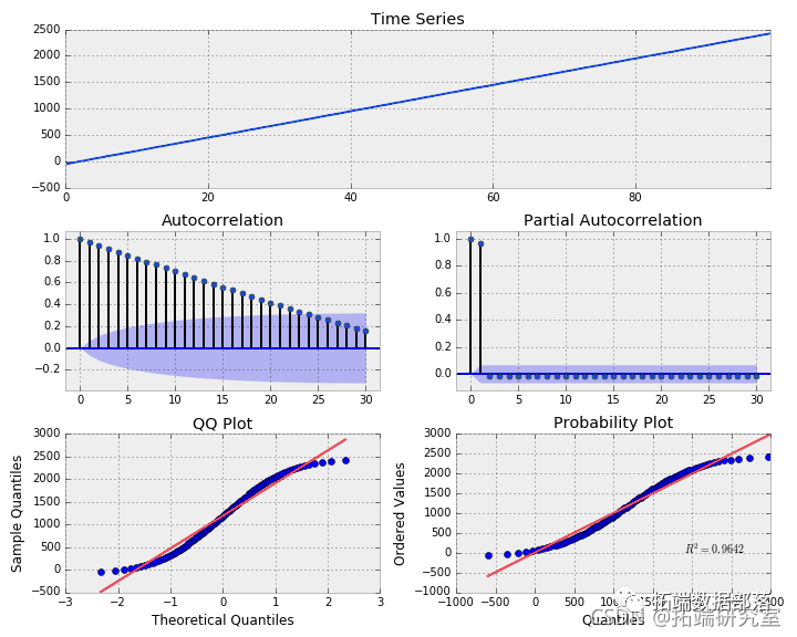

Simulating Linear Trend Model

Here we can see that the model’s residuals are correlated and linearly decrease as a function of lag. The distribution approximates normal. Before using this model for predictions, we must consider and eliminate the significant autocorrelation present in the sequence. The significance at lag 1 in the PACF suggests that an autoregressive model may be appropriate.

Log-Linear Models

These models are similar to linear models, except that the data points form an exponential function, representing a constant rate of change relative to each time step. For example, ABC company’s sales increase by X% in each time step. When plotting the simulated sales data, you would get a curve that looks like this.

# Simulating exponential growth for ABC
# Dates
pdat_rge('2007-01-01', '2012-01-01', freq='M')

# Assume sales grow exponentially
ale = [exp(x/12) for x inage1, len(id)+1)]

# Create dataframe and plot
df = d.ataame(sals, ix=x)
plt()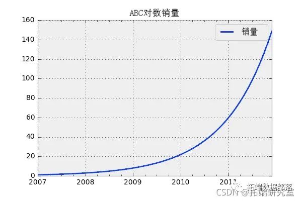

Simulating Exponential Function

Then we can transform the data by taking the natural logarithm of the sales. Now we can fit the data with linear regression.

# ABC log sales
indexid.plot()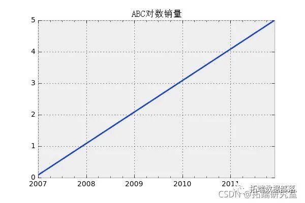

Natural Log of Exponential Function

As mentioned earlier, these models have a fatal weakness. They assume continuously uncorrelated errors, as we saw in the linear model example. In real life, TS data often violate our stationarity assumptions, which leads us to autoregressive models.

Autoregressive Models – AR(p)

When the dependent variable is regressed against one or more of its own lagged values, the model is called an autoregressive model. The formula is as follows:

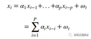
AR (P) Model

When you describe the model’s “order,” such as the order “p” of the AR model, p represents the number of lagged variables used in the model. For example, the AR(2) model or second-order autoregressive model is as follows:

AR (2) Model

Here, alpha (a) is the coefficient, and omega (w) is the white noise term. In AR models, alpha cannot equal 0. Note that the AR(1) model with alpha set to 1 is a random walk, and thus is not stationary.

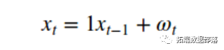
AR(1) Model, ALPHA = 1; Random Walk

Let’s simulate an AR(1) model with alpha set to 0.6.

# Simulating an AR(1) process with α=0.6
rndm.sed(1)
n_sams = int(1000)
a = 0.6
x = w = n.amma(siz=_apes)

for t in rane(n_saps):
    x[t] = a*x[t-1] + w[t]
    
plot(x, gs=lgs)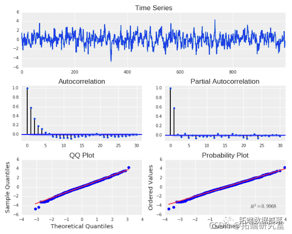

AR(1) Model, ALPHA = 0.6

As expected, the distribution of our simulated AR(1) model is normal. There is significant serial correlation between lagged values, especially at lag 1, as shown in the PACF plot.

Now we can fit an AR(p) model using Python’s statsmodels. First, we will fit the AR model to our simulated data and estimate the alpha coefficient of returns. Then we use the statsmodels function “order()” to see if the fitted model selects the correct lag. If the AR model is correct, the estimated alpha coefficient will be close to our true alpha of 0.6, and the selected order will equal 1.

# Fitting AR(p) model to simulated AR(1) model, alpha=0.6
md = AR(x).itm=30, ic='aic', trnd='nc')
%time st_oer = mt.R(x).stor(
    mxag=30, ic='aic', trnd='nc')

tuerer = 1

It seems we are able to recover the underlying parameters of the simulated data. Let’s simulate an AR(2) process with alpha_1 = 0.666 and alpha_2 = -0.333. For this, we use the statsmodel’s “generate_samples()” function. This function allows us to simulate AR models of any order.

# Simulating an AR(2) process

n = int(1000)

# Python requires us to specify zero lag values, which is 1
# Also note that the letters of the AR model must be negative
# For AR(p) models, we will also set the betas of MA to 0
ar = nr_[1, -ahas]
ma = npr_[1, beas]
ar2 = smt.arme_pe(ar=ar, ma=a, nsale=n) 
plot(ar2, lags=lags)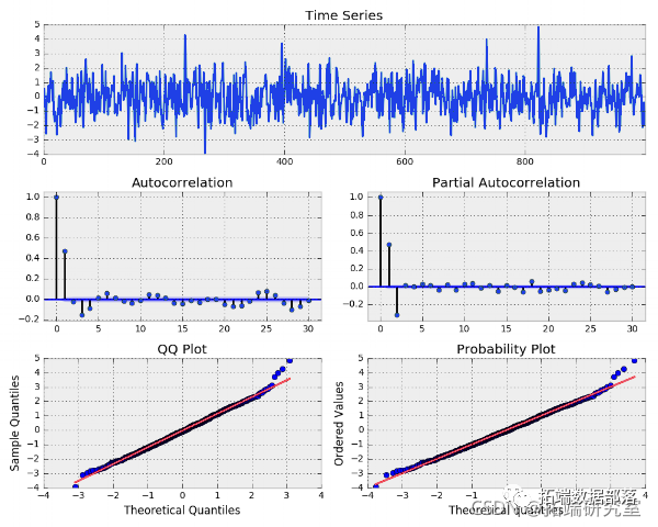

AR(2) Simulation ALPHA_1 = 0.666 and ALPHA_2 = -0.333

Let’s see if we can recover the correct parameters.

# Fitting AR(p) model to simulate AR(2) process

max_lag = 10
est_rer = st.AR(r2)sennc')

tu_rder = 2

Let’s see how the AR(p) model will fit the log returns of MSFT. This is the return TS.

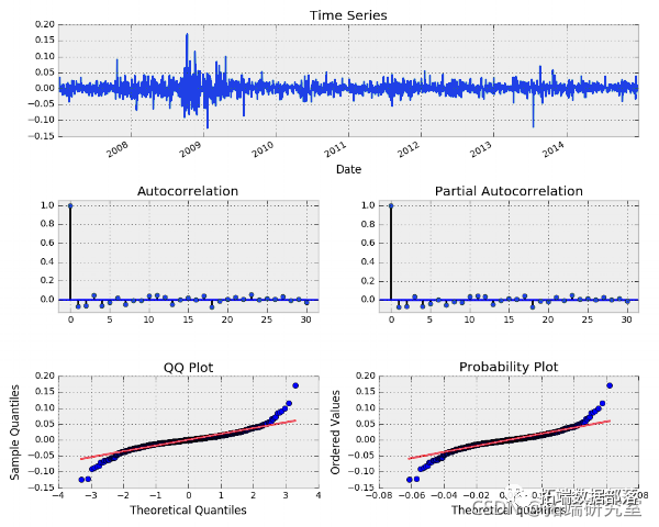
MSFT Log Return Time Series

# Selecting the best lag order for MSFT returns

max_ag = 30
ml = smt.AR(ls.MSFT).fit(mam_lg, c='aic', tnc)
es_rr = tAR(rts.FT).secter(
    maag=malag ic=aic', re=nc')
p('Best estimated lag order = {}'.format(etoer))

The best order is 23 lags or 23! Any model with so many parameters is unlikely to be useful in practice. Clearly, the complexity behind the return process is much more than this model can explain.

Moving Average Models – MA(q)

The MA(q) model is very similar to the AR(p) model. The difference is that the MA(q) model is a linear combination of past white noise error terms, rather than a linear combination of past observations like the AR(p) model. The purpose of the MA model is that we can directly observe the “shocks” in the error process by fitting the model to the error terms. In the AR(p) model, these shocks are indirectly observed through the ACF of a series of past observations. The formula for the MA(q) model is:

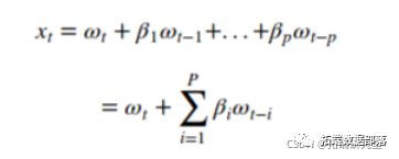
Omega (w) is white noise, with E(wt) = 0 and variance equal to sigma squared. Let’s simulate this process using beta=0.6 and specify the AR(p) alpha equal to 0.

# Simulating an MA(1) process

n = int(1000)

# Set AR(p) alphas equal to 0
alpas = npray([0.])
beas = np.ra([0.6])

# Add zero lag
ar = np_[1, -alph]
ma = np_[1, beta]
a1 = st.m_gerse(ar=ar, ma=a, naple=n) 
plot(ma1, lags=30)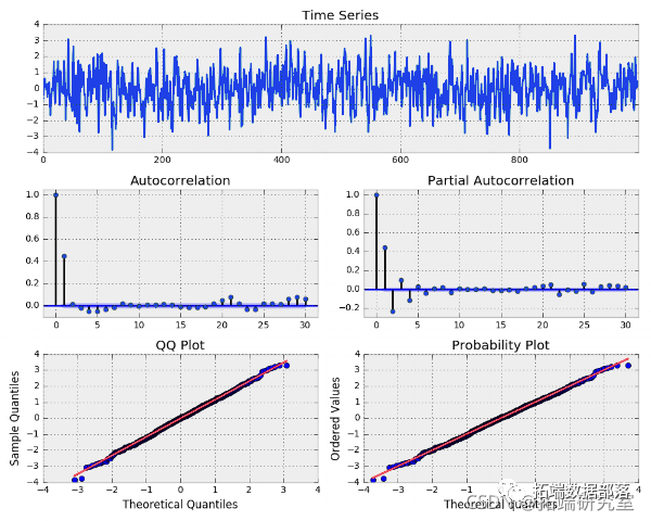

Simulated MA(1) Process with BETA=0.6

The ACF function shows that lag 1 is important, indicating that the MA(1) model may be suitable for our simulated series. When the ACF shows significance only at lag 1, I am unsure how to interpret the significance shown at lags 2, 3, and 4 in the PACF. We can now try to fit the MA(1) model to our simulated data. We can use the “ARMA()” function to specify the order we choose. We call its “fit()” method to return the model output.

# Matching MA(1) model with our simulated time series
# Specify ARMA model, order=(p, q).

maxlag = 30
st.RMa1, orer=(0,1)).fit
    maag=maxg, ethod='e', tren='nc')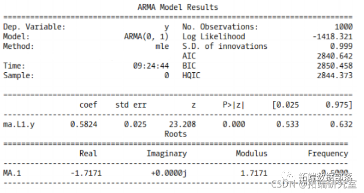

MA(1) Model Summary

The model is able to correctly estimate the lag coefficients, as 0.58 is close to our true value of 0.6. Also, note that our 95% confidence interval does indeed contain the true value. Let’s try simulating an MA(3) process, then fit a third-order MA model to the series and see if we can recover the correct lag coefficients (β). Beta 1-3 are equal to 0.6, 0.4, and 0.2, respectively.

# Simulating MA(3) process, beta=0.6, 0.4, 0.2

n = nt(100)
ar = nr_[1, -ahas]
ma = np.r_[1, betas]

m3 = genrae_sle(ar=ar, ma=ma, sple=n)
plot(ma3, las=30)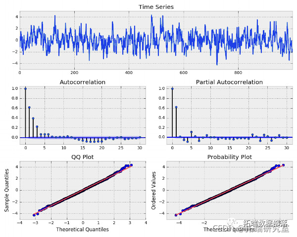

BETAS = [0.6, 0.4, 0.2] Simulated MA(3) Process

# Fitting MA(3) model to simulated time series

maxlg = 30
ARMA(ma3, order=(0, 3)).fit(
    xla=mx_ag, mehd='le',tred=nc').summary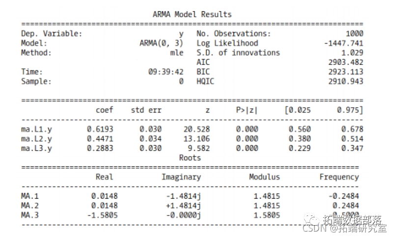

MA(3) Model Summary

The model is able to effectively estimate the actual coefficients. Our 95% confidence intervals also contain the true parameter values of 0.6, 0.4, and 0.2. Now let’s try fitting the MA(3) model to the log returns of SPY. Remember, we do not know the true parameter values.

# Fitting MA(3) to SPY returns

x_ag = 30
Y = lrsSY
ARMA(Y, ordr=(0, 3)).it(
    mlg=m_lg, thd'le', rndn'.summry())
plot(md.rsd lgs=m_lg)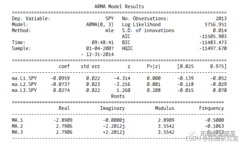

SPY MA (3) Model Summary

Let’s take a look at the model residuals.

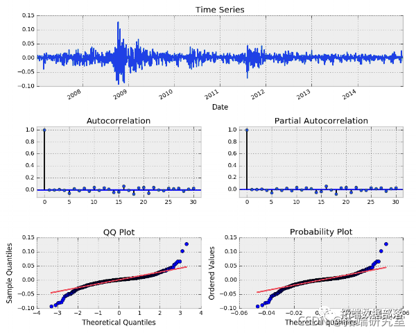
Nice. Some ACF lags have minor issues, especially at 5, 16, and 18. This could be sampling error, but combined with heavy tails, I think this is not the best model for predicting future SPY returns.

Autoregressive Integrated Moving Average Model – ARIMA(p, d, q)

ARIMA is a natural extension of the ARMA model class. As mentioned earlier, many of our TS are not stationary, but they can become stationary through differencing. We saw an example when we took the first difference of a Gaussian random walk and showed that it equals white noise. In other words, we took a non-stationary random walk and transformed it into stationary white noise through first differencing.

Without delving too deeply into this equation, just know that “d” refers to the number of times we difference the sequence. By the way, in Python, if we need to difference a sequence multiple times, we must use the np.diff() function. The pandas functions DataFrame.diff()/Series.diff() only handle the first difference of the dataframe/series and do not implement the recursive differencing needed in TSA.

In the example below, we iterate through a non-significant number of combinations of (p, d, q) orders to find the best ARIMA model for SPY returns. We use AIC to evaluate each model. The lowest AIC wins.

# Applying ARIMA(p, d, q) model to SPY returns
# Selecting the best order and final model based on AIC

for i in prng:
    for d in rng:
        for j in prng:
            try:
                tp_dl = ARIMAfit(lrs, orer=(i,d,j))
                if tpaic < betaic:
                    bestic = tmp_ic
                    bes_orer = (i, d, j)
                    bestl = tpmdl

# Residual plot of ARIMA model
plot(resid, lags=30)

It is not surprising that the difference of the best model is 0. Recall that we calculated stock returns using the first difference of log prices. Below, I plot the model residuals. The results are essentially the same as the ARMA(4, 4) model we fitted above. Clearly, this ARIMA model also does not explain the conditional volatility in the sequence!

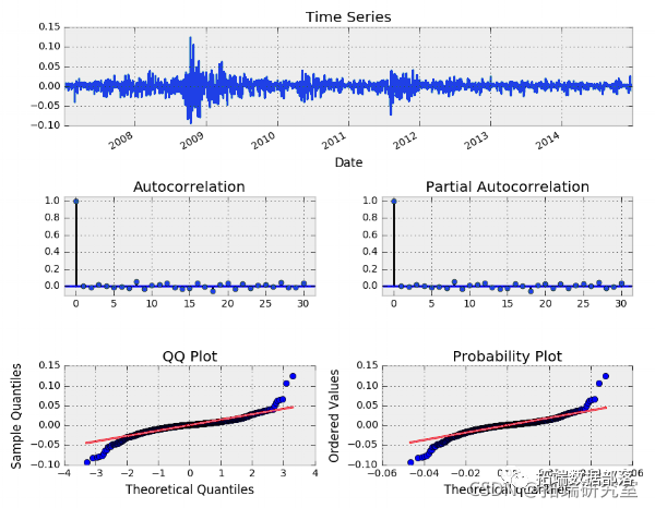
Fitting ARIMA Model to SPY Returns

Now we have at least accumulated enough knowledge to make simple predictions about future returns. Here we use the predict() method of our model. As parameters, the number of time steps to predict requires an integer, and the alpha parameter needs a decimal to specify the confidence interval. The default is set to 95% confidence. For 99%, set alpha to 0.01.

# Creating a 21-day SPY return forecast with 95%, 99% CI
n_steps = 21

fc9 =atFae(ncolmack([c99])
                     inx=clus=['wr_ci99', upr_ci_99')
fc_ll.head(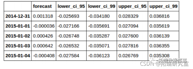

# Plotting 21-day SPY return forecast

ilc[-500:].cpy()

# In-sample forecast
prdct(side[0], t.id[-1])

plt(ax=x, stye=styes)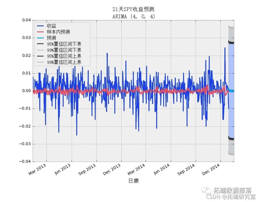

21-Day SPY Return Forecast – ARIMA(4,0,4)

Autoregressive Conditional Heteroskedasticity Model – ARCH(p)

The ARCH(p) model can simply be thought of as an AR(p) model applied to the variance of the time series. Another way to think about it is that the variance of our time series _at time t_ depends on past observations of the variance from previous periods.

ARCH(1) Model Formula

Assuming the mean of the series is zero, we can express the model as:

Zero Mean ARCH(1) Model

# Simulating ARCH(1) series
# Var(yt) = a_0 + a_1*y{t-1}**2
# If a_1 is between 0 and 1, then yt is white noise

Y = np.epy_lik

for t in rng(ln()):
    Y[t] = w[t] * sqrt((a0 + a1*y[t-1]**2)
# Simulated ARCH(1) series looks like white noise
plot(Y, lags=30)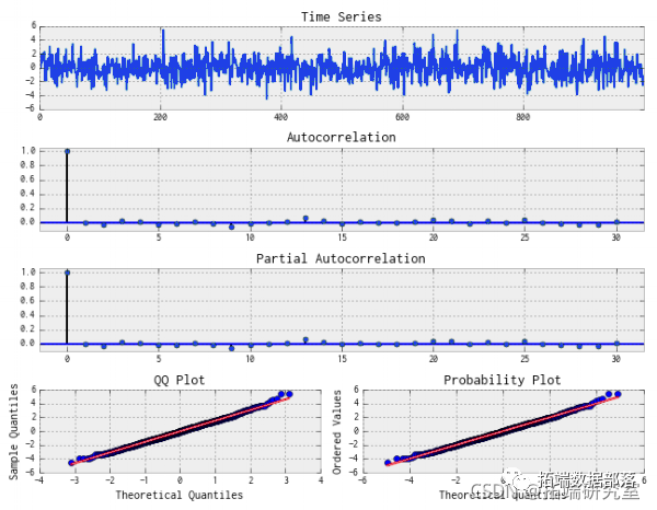

Simulated ARCH(1) Process

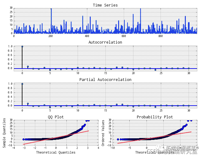
Simulated ARCH(1)**2 Process

Note that the ACF and PACF seem to show significance at lag 1, indicating that the AR(1) model for the variance may be appropriate.

Generalized Autoregressive Conditional Heteroskedasticity Model – GARCH(p,q)

Simply put, GARCH(p, q) is an ARMA model applied to the variance of the time series, meaning it has an autoregressive term and a moving average term. The AR(p) models the variance (squared errors) of the residuals, or simply the square of our time series. The MA(q) part models the variance of the process. The basic GARCH(1, 1) formula is:

GARCH(1, 1) Formula

Omega (w) is white noise, and alpha and beta are the parameters of the model. Additionally, alpha_1 + beta_1 must be less than 1; otherwise, the model is unstable. We can simulate a GARCH(1, 1) process below.

# Simulating a GARCH(1, 1) process

n = 10000
w = rnom.ral(sze=n)
eps = np.er_ike(w)
gsq =pzslie(w)

for i in rne1, n):
    sis[i] = a+ a1*(eps[i-1]**2) + b1*siq[i-1]
    es[i] = w[i] * srt(sisq[i])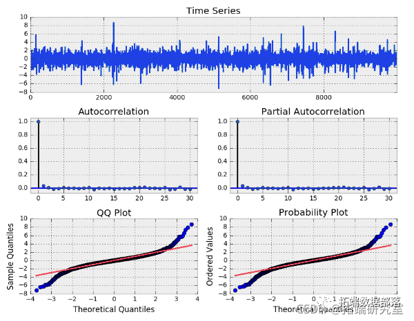

Simulating GARCH(1, 1) Process

Again, note that overall this process looks very similar to white noise; however, when we look at the squared eps sequence, take a look.

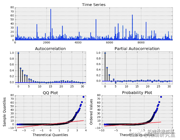
Simulated GARCH(1, 1) Squared Process

There is clearly autocorrelation, and the significance of the lags in the ACF and PACF indicates that our model needs AR and MA. Let’s see if we can recover our process parameters using the GARCH(1, 1) model. Here we use the arch_model function from the ARCH package.

# Matching GARCH(1, 1) model with our simulated EPS sequence
# We use the arch function

am = arch(ps)
fit(dae_freq=5)
summary())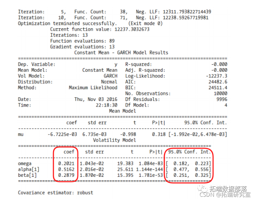

GARCH Model Fit Summary

Now let’s run an example using SPY returns. The process is as follows:

• Iterate through combinations of ARIMA(p, d, q) models to fit our time series.

• Select the GARCH model order based on the lowest AIC of the ARIMA model.

• Fit the GARCH(p, q) model to our time series.

• Check the autocorrelation of the model residuals and the squared residuals.

Also, note that I chose a specific time period to better highlight key points. However, results will vary depending on the time period studied.

    for i in pq_g:
        for d in d_ng:
            for j in p_ng:
                try:
                    tpml = ARIMA(T,order(i,d,j).fi
                    
                    if tmp_aic < best_aic:
                        best_ic =mpac
                        best_oder = (i, d, j)
                        best_ml =tm_ml

# Note that I have chosen a specific time period to run this analysis
bstmoel(TS)

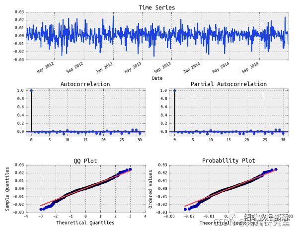
Fitting ARIMA(3,0,2) Model Residuals for SPY Returns

It looks like white noise.

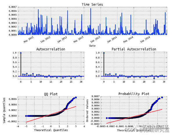
Fitting Squared Residuals of ARIMA(3,0,2) Model for SPY Returns

The squared residuals show autocorrelation. Let’s fit a GARCH model.

# Now we can fit the arch model using the parameters of the best fitting arima model

p_ = bst_dr
o= st_orde
q = bst_er

# Using Student's T distribution usually provides a better fit
arcd(TS, p=p_, o=o_, q=q_, 'StdensT')
fit(uat_eq=5, sp='ff')

summary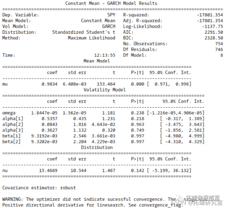

GARCH(3, 2) Model Fit for SPY Returns

When dealing with very small numbers, convergence warnings may occur. When necessary, multiplying the numbers by a coefficient of 10 to expand the magnitude can help, but for this demonstration, it is not necessary. Below are the residuals of the model.

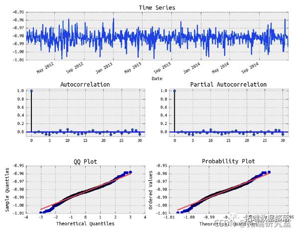
Fitting Residuals of GARCH(3, 2) Model for SPY Returns

Above looks like white noise. Now let’s look at the ACF and PACF of the squared residuals.

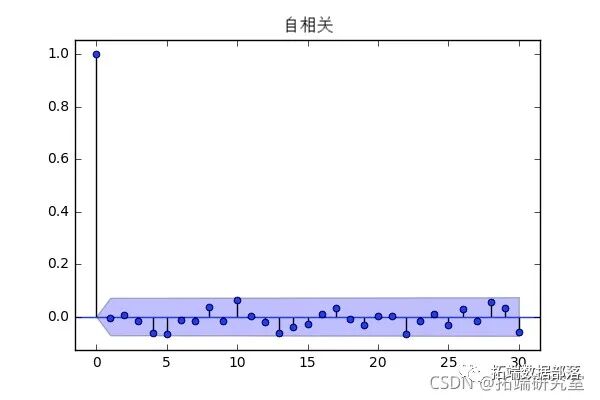
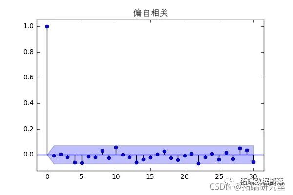
We have achieved a good model fit as the squared residuals show no significant autocorrelation.

Click the end of the article “Read the original”

to obtain the complete data..

This article is excerpted from Forecasting Stock Market Returns Using ARIMA and GARCH Models in Python.

Click the title to check past content

Time Series Analysis Models in R: ARIMA-ARCH/GARCH Model Analysis of Stock PricesR Language ARIMA-GARCH Volatility Model Forecasting Stock Market Daily Returns Time SeriesTime Series Analysis Models in R: ARIMA-ARCH/GARCH Model Analysis of Stock PricesR Language Multivariate Copula GARCH Model Time Series ForecastingPython Copula: Frank, Clayton, and Gumbel Copula Model Estimation and VisualizationR Language Copula GARCH Model Fitting Time Series and Simulation AnalysisMatlab Using Copula Simulation to Optimize Market Risk Data VaR AnalysisR Language Multivariate Copula GARCH Model Time Series ForecastingR Language Copula Function Stock Market Correlation Modeling: Simulating Random WalkR Language Implementing Copula Algorithm Modeling Dependency Case Study ReportR Language ARMA-GARCH-COPULA Model and Financial Time Series CaseR Language Bayesian Hierarchical Mixture Model Diagnostic Accuracy Study Based on CopulaR Language COPULA and Financial Time Series CaseMatlab Using Copula Simulation to Optimize Market Risk Data VaR AnalysisMatlab Using Copula Simulation to Optimize Market RiskR Language Multivariate Copula GARCH Model Time Series ForecastingR Language Bayesian Nonparametric MCMC Estimation of CopulaR Language COPULAS and Financial Time SeriesR Language Multiplicative GARCH Model for Volatility Forecasting of High-Frequency Trading DataR Language GARCH-DCC Model and DCC (MVT) Modeling EstimationPython Using GARCH, EGARCH, GJR-GARCH Models and Monte Carlo Simulation for Stock Price ForecastingR Language Time Series GARCH Model Analysis of Stock Market VolatilityR Language ARMA-EGARCH Model, Ensemble Forecasting Algorithm for SPX Actual Volatility ForecastingMatlab Implementing MCMC Markov Switching ARMA-GARCH Model EstimationPython Using GARCH, EGARCH, GJR-GARCH Models and Monte Carlo Simulation for Stock Price ForecastingUsing R Language for ARIMA + GARCH Trading Strategy on S&P 500 Stock IndexR Language Modeling Financial Time Series Data with Multivariate ARMA, GARCH, EWMA, ETS, Stochastic Volatility SV ModelsR Language Stock Market Index: ARMA-GARCH Model and Exploratory Analysis of Log Return DataR Language Multivariate Copula GARCH Model Time Series ForecastingR Language Using Multivariate AR-GARCH Model to Measure Market RiskTime Series Analysis Models in R: ARIMA-ARCH/GARCH Model Analysis of Stock PricesR Language Analyzing Stock Prices with Garch Model and Regression ModelComparison of GARCH (1,1), MA and Historical Simulation Method for VaRMatlab Estimating ARMA GARCH Conditional Mean and Variance ModelsR Language ARMA-GARCH-COPULA Model and Financial Time Series Case