1 What is an Operational Amplifier
An operational amplifier (op-amp) is used to regulate and amplify analog signals. An op-amp is an integrated device that contains multiple stages of amplification circuits, as shown in the figure:
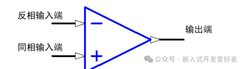
The left image shows the in-phase configuration, where the Vn terminal is grounded or at a stable level. When the Vp terminal level rises, the output Vo level rises; when the Vp terminal level falls, the output Vo level falls. The right image shows the inverting configuration, where the Vp terminal is grounded or at a stable level. When the Vn terminal level rises, the output Vo level falls; when the Vn terminal level falls, the output Vo level rises.

2 Properties of Operational Amplifiers
An ideal operational amplifier possesses the following properties:
Infinite input impedance: An ideal operational amplifier does not allow any current to flow into its input terminals, meaning the current signals at the input points V+ and V- are always zero, resulting in infinite input impedance.
Output impedance approaching zero: The output of an ideal operational amplifier acts as a perfect voltage source. Regardless of the current flowing to the amplifier’s load, the output voltage remains constant, resulting in zero output impedance.
Infinite open-loop gain: In an open-loop state, the differential signal at the input terminals has infinite voltage gain, making operational amplifiers highly suitable for practical applications with negative feedback configurations.
Infinite common-mode rejection ratio: An ideal operational amplifier only responds to the voltage difference between V+ and V- (differential signal), completely ignoring the common-mode signal (the same part of both input signals).
Common-mode signal: When both inputs are the same. Differential signal: When the two input signals are 180 degrees out of phase.
Integrated operational amplifiers can operate in two states:
Linear state and nonlinear state. When a negative feedback circuit is applied to the integrated operational amplifier, it operates in the linear state. If a positive feedback circuit is applied or it operates in an open-loop state, it operates in the nonlinear state.
Integrated operational amplifiers in the linear state have the following characteristics:
They exhibit virtual short-circuit characteristics, and the currents flowing into and out of the input terminals are both zero, I- = I+ = 0A.
They exhibit virtual short characteristics, where the voltages at the two input terminals are equal, U+ = U-.
Virtual short and virtual open:
Virtual short: The open-loop gain of the integrated operational amplifier is very high, typically above 80dB for general-purpose operational amplifiers. However, the output voltage of the op-amp is limited, usually between 10V and 14V. Since the differential input voltage of the op-amp is less than 1 mV, the two input terminals can be approximated as equal potential, similar to a short circuit. The greater the open-loop voltage gain, the closer the potentials at the two input terminals are to being equal, a characteristic known as virtual short.
Virtual open: Integrated operational amplifiers have high input impedance characteristics, with the input resistance of both the non-inverting and inverting terminals typically above 1MΩ. Therefore, the current flowing into the op-amp’s input terminals is often less than 1uA, much smaller than the current from the external circuit. Thus, the two input terminals can usually be treated as open, and the larger the input resistance of the op-amp, the closer the non-inverting and inverting terminals are to being open. When the op-amp is in the linear state, this characteristic allows the two input terminals to be treated as equivalent open circuits, referred to as virtual open.
Integrated operational amplifiers in the nonlinear state have the following characteristics:
When the voltage at the non-inverting input is greater than that at the inverting input, the output voltage is high.
When the voltage at the non-inverting input is less than that at the inverting input, the output voltage is low.
3 Classification of Operational Amplifiers
Operational amplifiers can be classified based on parameters as shown in the figure:
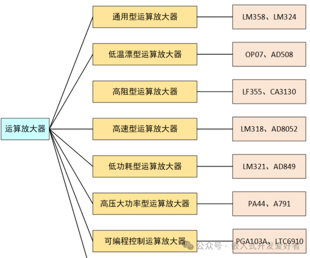
General-purpose operational amplifiers: Inexpensive, with performance specifications suitable for general applications, commonly used models include LM358 and LM324.
Low drift operational amplifiers: In precision instruments and weak signal detection in automatic control instruments, the offset voltage must be small and not vary with temperature changes, commonly used models include OP07 and AD508.
High precision operational amplifiers: Less affected by temperature, low noise, high sensitivity, suitable for small signal amplification, commonly used model is CF725M.
High impedance operational amplifiers: Very high differential input impedance, very low input bias current, typically Rid > 1GΩ ~ 1TΩ, with Ib in the range of a few picoamperes to tens of picoamperes, commonly used models include LF355 and CA3130.
High-speed operational amplifiers: High conversion rates and wide frequency response, used for fast A/D and D/A converters, commonly used models include LM318 and AD8052.
Low power operational amplifiers: Operate at low supply voltage and consume low power, commonly used models include LM321 and AD849.
High voltage high power operational amplifiers: The output voltage of the op-amp is limited by the power supply. To increase the output voltage or current, auxiliary circuits are usually required. High voltage high power op-amps can output high voltage and large current without any external current, commonly used models include PA44 and A791.
Programmable gain operational amplifiers: Gain can be varied, commonly used models include PGA103A and LTC6910.
4 Parameters of Operational Amplifiers
Common-mode input resistance: Represents the ratio of the input common-mode voltage range to the change in bias current within that range when the operational amplifier operates in the linear region.
DC common-mode rejection: Measures the operational amplifier’s ability to suppress the same DC signal applied to both input terminals.
AC common-mode rejection: Measures the operational amplifier’s ability to suppress the same AC signal applied to both input terminals.
Gain bandwidth product: A constant defined in the region where the open-loop gain decreases at (-20dB/decade) with frequency.
Input bias current: The average current flowing into the input terminals when the operational amplifier operates in the linear region.
Bias current temperature drift: The change in input bias current due to temperature variations.
Input offset current: The difference in current flowing into the two input terminals.
Input offset current temperature drift: The change in input offset current due to temperature variations.
Differential input resistance: The ratio of the change in input voltage to the corresponding change in input current, where the change in voltage causes a change in current.
Output impedance: The internal equivalent small-signal impedance at the output terminal when the operational amplifier operates in the linear region.
Output voltage swing: The maximum peak voltage swing that can be achieved without clipping the output signal.
Power consumption: The static power consumed at a given supply voltage.
Power supply rejection ratio: Measures the operational amplifier’s ability to maintain its output unchanged when the supply voltage varies.
Transition rate: The maximum ratio of the change in output voltage to the time required for that change.
Supply current: The static current consumed by the device at a specified supply voltage.
Unity gain bandwidth: The maximum operating frequency of the operational amplifier when the open-loop gain is greater than 1.
Input offset voltage: The voltage difference that must be applied at the input terminals to make the output voltage zero.
Input offset voltage temperature drift: The change in input offset voltage due to temperature variations.
Input capacitance: The equivalent capacitance at any input terminal when the operational amplifier operates in the linear region.
Input voltage range: The range of input voltages allowed for the operational amplifier to function normally.
Input voltage noise density: Can be viewed as a series noise voltage source connected to any input terminal.
Input current noise density: Can be viewed as two noise current sources connected to each input terminal and the common terminal.
5 Applications of Operational Amplifiers
Inverting amplifier circuit as shown:
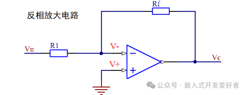
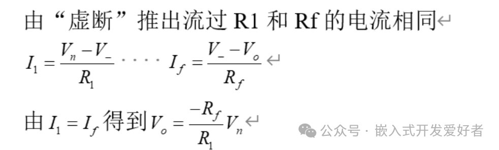
Relationship between input and output voltages of the inverting amplifier circuit:
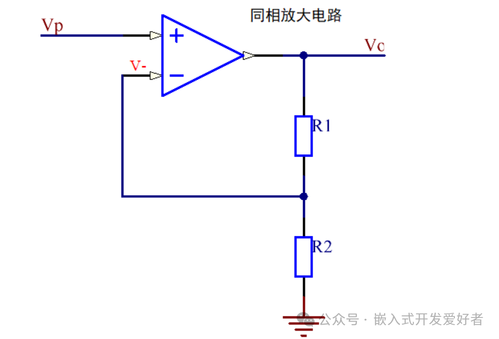
Non-inverting amplifier circuit as shown:
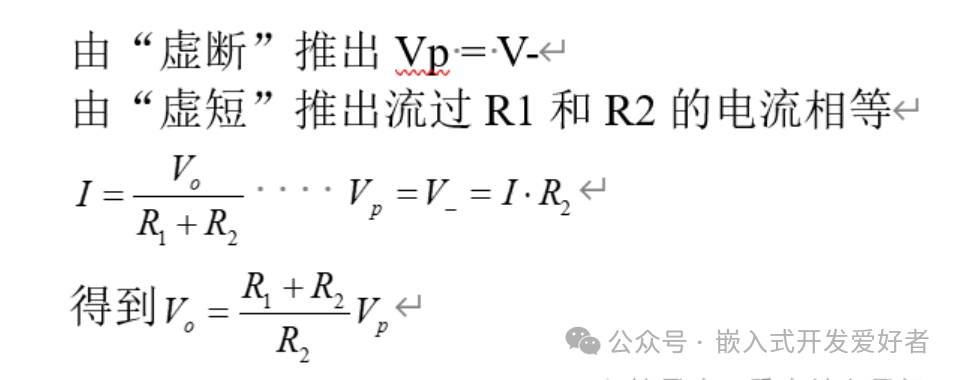
Relationship between input and output voltages of the non-inverting amplifier circuit:
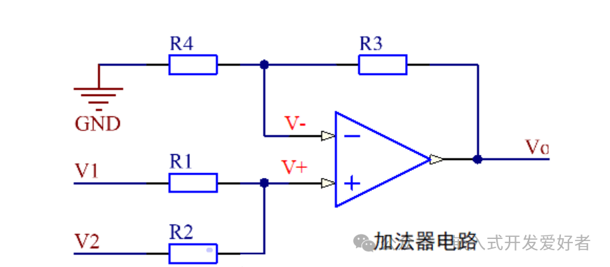
Summing circuit as shown:
Relationship between input and output voltages of the summing circuit:
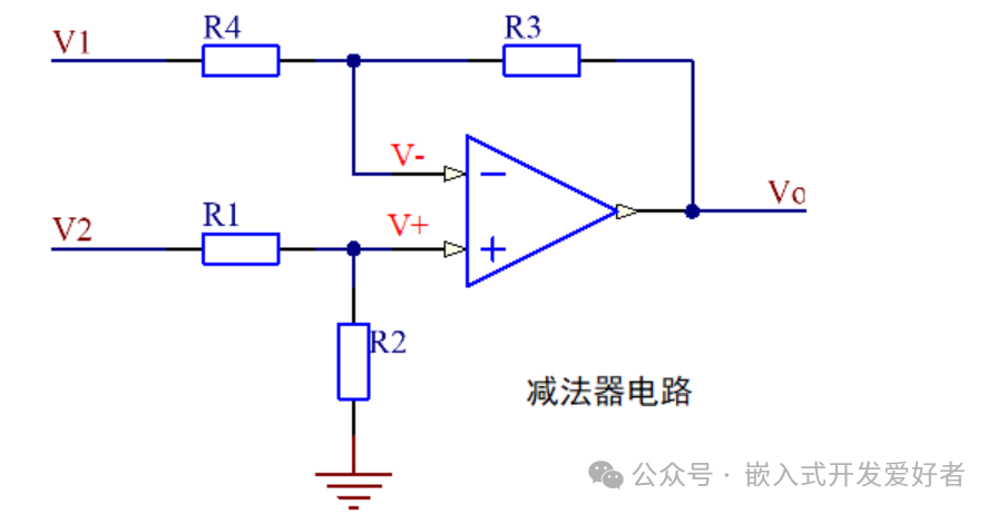
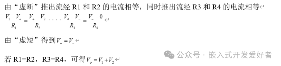 Subtraction circuit as shown:
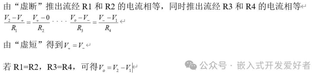
 Relationship between input and output voltages of the subtraction circuit:
 Integration circuit as shown: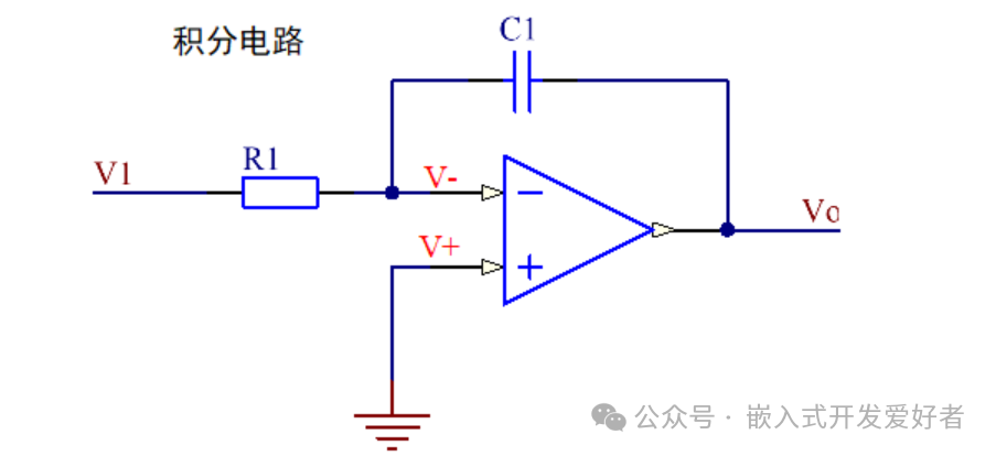
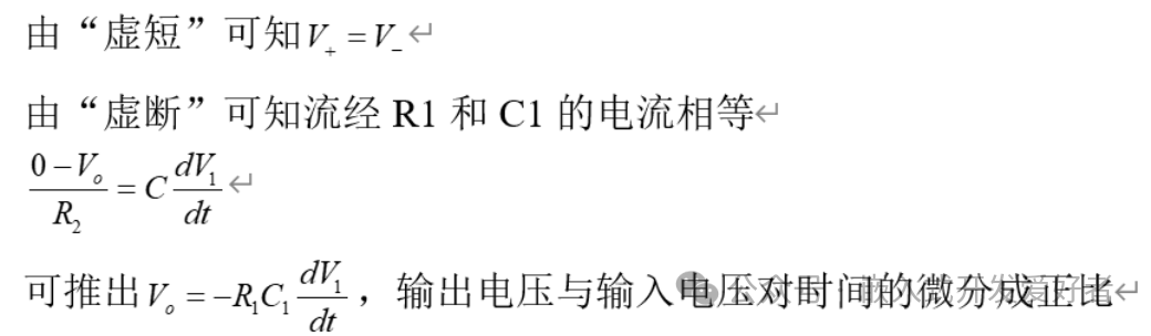
Relationship between input and output voltages of the differentiation circuit:
 Differential amplifier circuit as shown: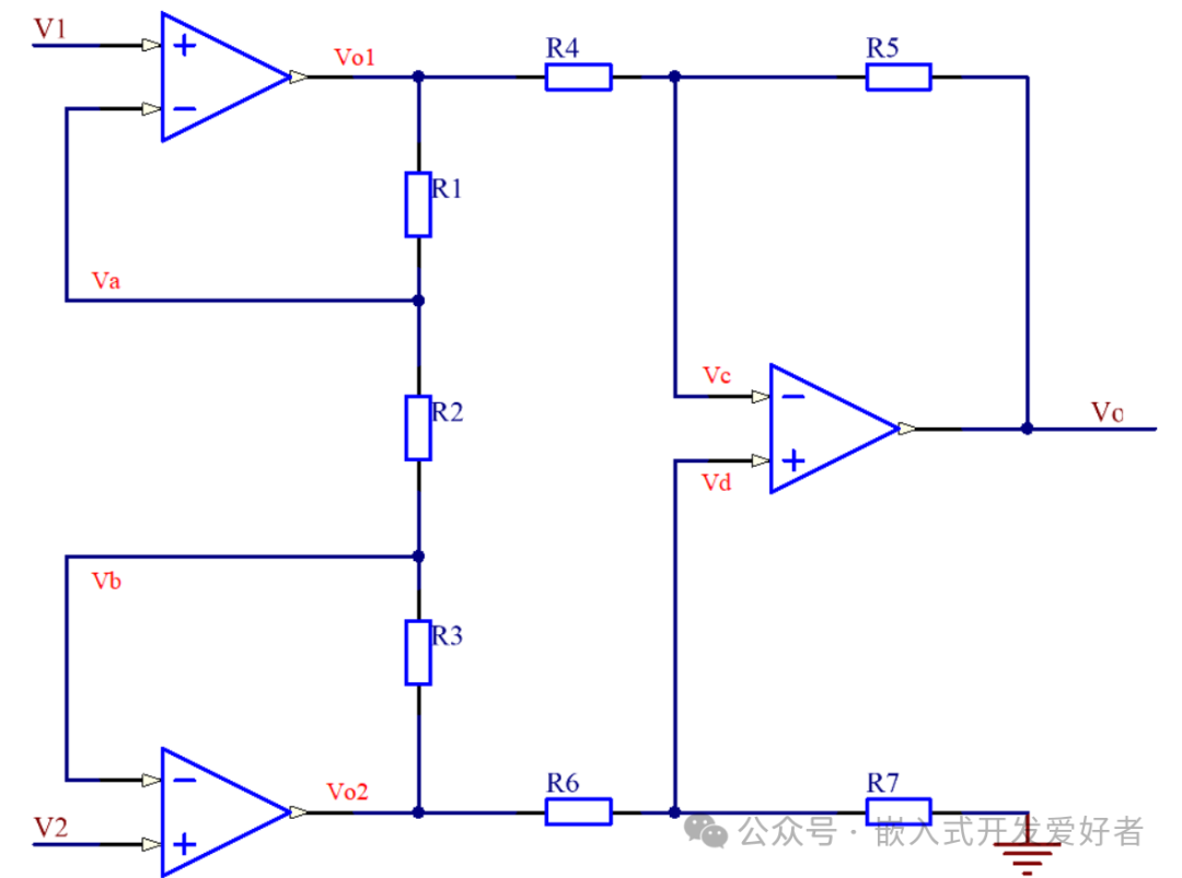
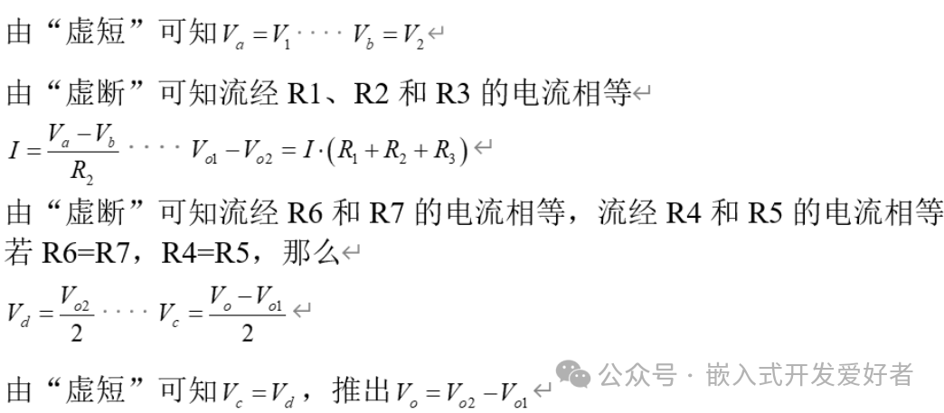
Relationship between input and output voltages of the differential amplifier circuit:
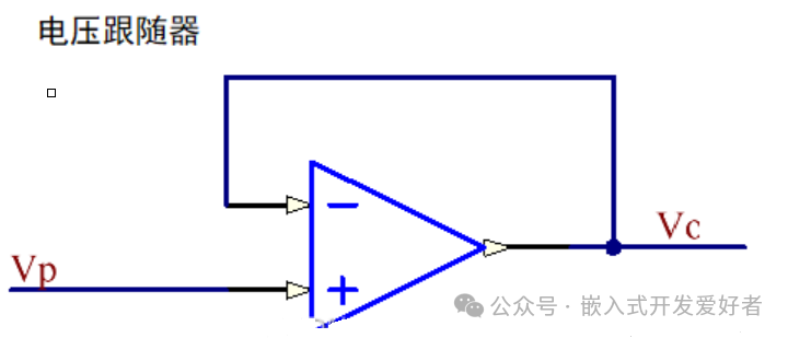
Voltage follower circuit as shown:
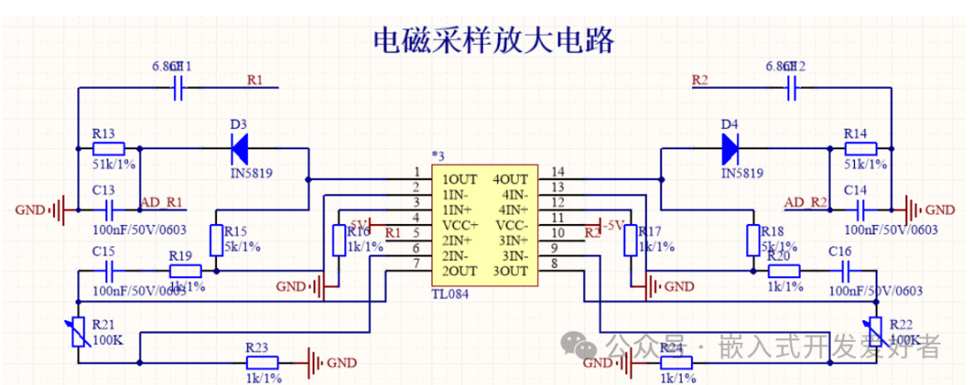
Electromagnetic sampling amplifier circuit as shown: